Concepts¶

FeatureByte Catalog¶

A FeatureByte Catalog operates as a centralized repository for organizing tables, entities, features, and feature lists and other objects to facilitate feature reuse and serving.

By employing a catalog, team members can effortlessly share, search, retrieve, and reuse these assets while obtaining comprehensive information about their properties.

Create multiple catalogs for data warehouses covering multiple domains to maintain clarity and easy access to domain-specific metadata.

SDK Reference

Refer to the Catalog object main page or to the specific links:

list catalogs,
create a catalog,
get the currently active catalog,
activate a catalog,
list tables, entities, features or feature lists in a catalog,
and retrieve a table, an entity, a feature or a feature list from a catalog.

User Interface

Learn by example with our 'Create Catalog' UI tutorials.

Source Table and Special Columns¶

Data Source¶

A Data Source object in FeatureByte represents a collection of source tables that the feature store can access. From a data source, you can:

Retrieve the list of databases available
Obtain the list of schemas within the desired database
Access the list of source tables contained in the selected schema
Retrieve a source table for exploration or registering it in the catalog.

SDK Reference

Refer to the DataSource object main page or to the specific links:

User Interface

Learn by example with our 'Register Tables' UI tutorials.

Source Table¶

A Source Table in FeatureByte is a table of interest that the feature store can access and is located within the data warehouse.

To register a Source Table in a FeatureByte catalog, first determine its type. There are four supported types: event table, item table, dimension table and slowly changing dimension table.

Note

Registering a table according to its type determines the types of feature engineering operations that are possible on the table's views and enforces guardrails accordingly.

To identify the table type and collect key metadata, Exploratory Data Analysis (EDA) can be performed on the source table. You can obtain descriptive statistics, preview a selection of rows, or collect additional information on their columns.

SDK Reference

Refer to the SourceTable object main page or to the specific links:

list source tables in a data source,
retrieve a source table from a data source,
obtain descriptive statistics,
and preview a selection of rows,

User Interface

Learn by example with our 'Register Tables' UI tutorials.

Primary key¶

A Primary Key is a column or set of columns uniquely identifying each record (row) in a table.

The primary key is used to enforce the integrity of the data and ensure no duplicate records in the table. The primary key must satisfy the following requirements:

Unique: Each record in the table must have a unique primary key value.
Non-null: The primary key cannot be null (empty) for any record.
Stable: The primary key value should not change over time.

Four types of primary keys can be found in FeatureByte tables:

Event ID: The primary key in Event table.
Item ID: The primary key in Item table.
Dimension ID: The primary key in Dimension table.
Surrogate key: The primary key in Slowly Changing Dimension (SCD) table.

Event ID¶

An event ID serves as the primary key of the Event table. An event ID in such a context entails:

Uniqueness: The event ID is unique for each row, ensuring that each business event recorded in the table can be distinctly identified. No two rows in the table will have the same event ID.
Representation of Business Events: Each row in the event table represents a business event. A business event could be anything significant to the business that needs to be recorded, like a transaction, a customer interaction, a system failure, etc.
Time Association: Along with the event ID, the table will typically include a timestamp, the event timestamp, indicating when the event occurred.

Item ID¶

An item ID, serving as the primary key in an Item table, plays a crucial role in organizing and relating detailed information about specific business events. An item ID in such a context entails:

Uniqueness: The item ID is unique for each row, ensuring that each item can be distinctly identified and accessed.
Detailed Event Information: While the event table records each occurrence of a business event with a timestamp, the item table delves into the specifics of these events. For instance, in a retail context, if the Event Table records a sale, the Item Table would list the individual products (items) that were part of that sale.
Implicit Time Link: Although the item table itself might not include a timestamp, its linkage to the event table, which does have a timestamp, implicitly associates each item with the time of the event. For example, a product item's details in the item table are connected to the timestamp of the sale event in the event Table.
One-to-Many Relationship with event ID: The item ID typically has a one-to-many relationship with the event ID. This means that one event ID (like a customer order) can correspond to multiple item IDs (various products in that order).

Example

Depending on the business context, the Item Table could include:

For product items in customer orders: Product ID, name, quantity, price, category, and other relevant details.
For drug prescriptions in doctor visits: Drug ID, name, dosage, frequency, prescribing doctor, and other pertinent information.

Dimension ID¶

A Dimension ID serves as the primary key in a Dimension table. This means it uniquely identifies each record or row in the table. Unlike event tables that typically store quantitative data (like sales figures, quantities), dimension tables store statitc qualitative information. Dimension IDs should be unique and stable over time. This ensures that historical data remains consistent and reliable.

Example

A product dimension table would store details about products, and each product would have a unique Dimension ID.

Surrogate key¶

In a Slowly Changing Dimension (SCD) table, a surrogate key is a unique identifier assigned to each record. It is used to provide a stable identifier even as the table changes over time.

Example

Consider a table that keeps track of customer addresses over time, known as a Slowly Changing Dimension (SCD) table. When a customer updates their address, a new record with the updated address is added rather than modifying the existing record. To uniquely identify each record, a surrogate key is used as the primary key. Additionally, an effective timestamp is included to indicate when the address change occurred.

In this table, the Customer ID acts as the natural key, connecting records to a specific customer. The Customer ID alone does not guarantee uniqueness, as customers may have multiple addresses throughout time. But, each Customer ID is linked to only one address for a specific time period, enabling the table to preserve historical data.

Natural key¶

In a Slowly Changing Dimension (SCD) table, a natural key (also called alternate key) is a column that remains constant over time and uniquely identifies each active row in the table at any point-in-time.

This key is crucial in maintaining and analyzing the historical changes made in the table.

Example

Consider a SCD table providing changing information on customers, such as their addresses. The customer ID column of this table can be considered a natural key since:

it remains constant
uniquely identifies each customer

A given customer ID is associated with at most one address at a particular point-in-time, while over time, multiple addresses can be associated with a given customer ID.

Foreign key¶

A Foreign Key is a column or a group of columns in one table that refers to the primary key in another table. It establishes a relationship between two tables.

Example

An example of foreign key is Customer ID in an Orders table, which links it to the Customer table where Customer ID is the natural key.

Special Timestamp columns¶

Event Timestamp¶

The event timestamp column in an Event table records the exact time at which a specific event occurred.

Effective Timestamp¶

The Effective Timestamp column in a Slowly Changing Dimension (SCD) table specifies the time when the record becomes active or effective.

Example

If a customer changes their address, the effective timestamp would be the date when the new address becomes active.

Expiration Timestamp¶

The Expiration (or end) Timestamp column in a Slowly Changing Dimension (SCD) table specifies the time when the record is no longer valid or active.

Example

If a customer changes their address, the expiration timestamp would be when the old address is no longer valid.

Note

While this column is useful for data management, it cannot be used for feature engineering as it is related to information unknown during the inference time and may cause time leakage. For this reason, the column is discarded by default when views are generated from tables.

Record Creation Timestamp¶

A Record Creation Timestamp refers to the time when a particular record was created in the data warehouse. The record creation timestamp is usually automatically generated by the system when the record is first created, but a user or an administrator can manually set it.

Note

While this column is useful for data management, it is usually not used for feature engineering as it is sensitive to changes in data management that are usually unrelated to the target to predict. This also may cause feature drift and undesirable impact on predictions. For this reason, the column is discarded by default when views are generated from tables.

The information is, however, used to analyze the data availability and freshness of the tables to help with the configuration of their default feature job setting.

Time Zone Offset¶

A time zone offset, also known as a UTC offset, is a difference in time between Coordinated Universal Time (UTC) and a local time zone. The offset is usually expressed as a positive or negative number of hours and minutes relative to UTC.

Example

If the local time is 3 hours ahead of UTC, the time zone offset would be represented as "+03:00". Similarly, if the local time is 2 hours behind UTC, the time zone offset would be represented as "-02:00".

Note

When you register an Event table, you can specify a separate column that provides the time zone offset information. By doing so, all date parts transforms in the event timestamp column will be based on the local time instead of UTC.

The required format for the column is "(+|-)HH:mm".

Timestamp with Time Zone Offset¶

The Snowflake data warehouse supports a timestamp type with time zone offset information (TIMESTAMP_TZ). FeatureByte recognises this timestamp type and date parts for columns or features using timestamp with time zone offset are based on the local time instead of UTC.

Important

Timestamp columns that are stored without time zone offset information are assumed to be UTC timestamps.

Active Flag¶

The Active Flag (also known as Current Flag) column in a Slowly Changing Dimension (SCD) table is used to identify the current version of the record.

Example

If a customer changes their address, the active flag would be set to 'Y' for the new address and 'N' for the old address.

Note

While this column is useful for data management, it cannot be used for feature engineering as the value changes overtime and may differ between training and inference time. It may cause time leakage. For this reason, the column is discarded by default when views are generated from tables.

FeatureByte Tables¶

Table¶

A Table in FeatureByte represents a source table and provides a centralized location for metadata for that table. This metadata determines the type of operations that can be applied to the table's views.

Important

A source table can only be associated with one active table in the catalog at a time. This means that the active table in the catalog is the source of truth for the metadata of the source table. If a table in the catalog becomes deprecated, it can be replaced with a new table in the catalog that has updated metadata.

Table Registration¶

To register a table in a catalog, determine its type first. The table’s type will determine the types of feature engineering operations possible on the table's views and enforces guardrails accordingly. Currently, FeatureByte recognizes four table types:

Event Table: a table where each row indicates a unique business event occurring at a particular time.
Item Table: a table containing detailed information about a specific business event.
Slowly Changing Dimension Table (SCD): a table containing data that changes slowly and unpredictably over time.
Dimension Table: a table containing static descriptive data.

Two additional table types, Regular Time Series and Sensor data, will be supported shortly.

Optionally, you can include additional metadata at the column level after creating a table to support feature engineering further. This could involve tagging columns with related entity references, updating column description, tagging semantics or defining default cleaning operations.

SDK Reference

Refer to the Table object main page or to the specific links:

User Interface

Learn by example with our 'Register Tables' UI tutorials.

Event Table¶

An Event Table represents a table in the data warehouse where each row indicates a unique business event occurring at a particular time.

Examples

Event tables can take various forms, such as

An Order table in E-commerce
A Credit Card Transactions table in Banking
Doctor Visits in Healthcare
Clickstream on the Internet.

To create an Event Table in FeatureByte, it is necessary to identify two important columns in your data: the event ID and the event timestamp. The event ID is a unique identifier for each event, while the timestamp indicates when the event occurred.

Note

If your data warehouse is a Snowflake data warehouse, FeatureByte accepts timestamp columns that include time zone offset information.

For timestamp columns without time zone offset information or for non-Snowflake data warehouses, you can specify a separate column that provides the time zone offset information. By doing so, all date parts transforms in the event timestamp column will be based on the local time instead of UTC.

Additionally, the column that represents the record creation timestamp may be identified to enable an automatic analysis of data availability and freshness of the source table. This analysis can assist in selecting the default feature job setting that defines the scheduling of the computation of features associated with the Event table.

SDK Reference

Refer to the Table object main page or to the specific links:

User Interface

Learn by example with our 'Register Tables' UI tutorials.

Item Table¶

An Item Table represents a table in the data warehouse containing detailed information about a specific business event.

Examples

An Item table may contain information about:

Product Items purchased in Customer Orders
or Drug Prescriptions issued during Doctor Visits by Patients.

Typically, an Item table has a 'one-to-many' relationship with an Event table. Despite not explicitly including a timestamp, it is inherently linked to an event timestamp through its association with the Event table.

To create an Item Table, it is necessary to identify the columns that represent the item ID and the event ID and determine which Event table is associated with the Item table.

SDK Reference

How to register an item table.

User Interface

Learn by example with our 'Register Tables' UI tutorials.

Slowly Changing Dimension (SCD) Table¶

An SCD Table represents a table in a data warehouse that contains data that changes slowly and unpredictably over time.

There are two main types of SCD Tables:

Type 1: Overwrites old data with new data
Type 2: Maintains a history of changes by creating a new record for each change.

FeatureByte only supports using Type 2 SCD Tables since Type 1 SCD Tables may cause data leaks during model training and poor performance during inference.

A Type 2 SCD Table utilizes a natural key to distinguish each active row and facilitate tracking of changes over time. The SCD table employs effective and end (or expiration) timestamp columns to determine the active status of a row. In certain instances, an active flag column may replace the expiration timestamp column to indicate whether a row is active.

Example

Here is an example of a Type 2 SCD table for tracking changes to customer information:

Customer ID	First Name	Last Name	Address	City	State	Zip Code	Valid From	Valid To
123456	John	Smith	123 Main St	San Francisco	CA	12345	13/01/2019 11:00:00	16/03/2021 10:00:00
123456	John	Smith	456 Oak St	Oakland	CA	67890	16/03/2021 10:00:00	NULL
789012	Jane	Doe	789 Maple Ave	New York City	NY	34567	15/09/2020 10:00:00	NULL

In this example, each row represents a specific version of customer information. The customer entity is identified by the natural key "Customer ID". If a customer's information changes, a new row is added to the table with the updated information, along with an effective timestamp ("Valid From" column) and end timestamp ("Valid To" column) to indicate the period during which that version of the information was active. The end timestamp is NULL for the current version of the information, indicating that it is still active.

For example, the customer with ID 123456 initially had an address of 123 Main St in San Francisco, CA, but then changed his address to 456 Oak St in Oakland, CA on 16/03/2021. This change is reflected in the SCD table by adding a new row with the updated address and Valid From of 16/03/2021 10:00:00, and a Valid To with the same timestamp for the previous version of the address.

To create an SCD Table in FeatureByte, it is necessary to identify columns for the natural key, effective timestamp, optionally surrogate key, end (or expiration) timestamp, and active flag.

SDK Reference

How to register a SCD table.

User Interface

Learn by example with our 'Register Tables' UI tutorials.

Dimension Table¶

A Dimension Table represents a table in the data warehouse containing static descriptive data.

Important

Using a Dimension table requires special attention. If the data in the table changes slowly, it is not advisable to use it because these changes can cause significant data leaks during model training and adversely affect the inference performance. In such cases, it is recommended to use a Type 2 Slowly Changing Dimension table that maintains a history of changes.

To create a Dimension Table in FeatureByte, it is necessary to identify which column represents its primary key, also referred in FeatureByte as the dimension ID.

SDK Reference

How to register a dimension table.

User Interface

Learn by example with our 'Register Tables' UI tutorials.

Table Status¶

When a table is registered in a catalog, its status is set to 'PUBLIC_DRAFT' by default. Once the table is prepared for feature engineering, you can modify its status to 'PUBLISHED'. If a table needs to be deprecated, you can update its status to 'DEPRECATED'.

SDK Reference

How to:

User Interface

Learn by example with our 'Manage feature life cycle' UI tutorials.

Table Columns Metadata¶

Table Column¶

A Table Column refers to a specific column within a table. You can add metadata to the column to help with feature engineering, such as tagging the column with entity references, updating column description, tagging semantics or defining default cleaning operations.

SDK Reference

Refer to the TableColumn object main page or to the specific links:

update_description,
tag an entity to a column,
obtain descrpitive statistics for a column,
and specify default cleaning operations.

User Interface

Learn by example with our 'Add descriptions and Tag Semantics' and Set Default Cleaning Operations UI tutorials.

Entity Tagging¶

The Entity Tagging process involves identifying the specific columns in tables that identify or reference a particular entity.

These columns are typically primary keys, natural keys, or foreign keys of the table, but not necessarily.

Example

Consider a database for a company that consists of 2 SCD tables: one table for employees and one table for departments. In this database,

the natural key of the employees table identifies the Employee entity.
the natural key of the department tables identifies the Department entity.
the employees table may also have a foreign key column referencing the Department entity.

SDK Reference

How to tag a column with an entity reference.

User Interface

Learn by example with our 'Register Entities' UI tutorials.

Cleaning Operations¶

Cleaning Operations determine the procedure for cleaning data in a table column before performing feature engineering. The cleaning operations can either be set as a default operation in the metadata of a table column or established when creating a view in a manual mode.

These operations specify how to manage the following scenarios:

Missing values
Disguised values
Values that are not in an anticipated list
Numeric values and dates that are out of boundaries
String values when numeric values are expected

If changes occur in the data quality of the source table, new versions of the feature can be created with new cleaning operations that address the new quality issues.

Important Note for FeatureByte Enterprise Users

In Catalogs with Approval Flow enabled, changes in table metadata initiate a review process. This process recommends new versions of features and lists linked to these tables, ensuring that new models and deployments use versions that address any data issues.

SDK Reference

How to:

set default cleaning operations for a column,
create a view in a manual mode,
create a new feature version with new cleaning operations.

User Interface

Learn by example with our 'Set Default Cleaning Operations' and 'Manage feature life cycle' UI tutorials.

Column Semantics¶

Recognizing the semantics of data fields and tables is essential for effective and reliable feature engineering. Without this understanding, there's a risk of creating irrelevant or misleading features, and missing out on key insights. Here are some examples of common errors due to misunderstanding data semantics:

Incorrectly applying 'sum' to intensity measurements, like patient temperatures in a doctor's visit table.
Misinterpreting a weekday column as numerical and using inappropriate operations like sum, average, or max, instead of more suitable ones like count per weekday, most frequent weekday, weekdays entropy, or unique count.

To guide users in choosing the right feature engineering techniques, FeatureByte introduces a semantic layer for each registered table. This layer encodes the semantics of data fields using a specially designed data ontology, tailored for feature engineering.

FeatureByte Copilot assists in this process for enterprise users. It uses Generative AI to analyze metadata from tables and columns and proposes semantic tags for each column. This semantic tagging is then used by FeatureByte Copilot to suggest relevant data aggregations, filters, and feature combinations during feature ideation.

User Interface

Learn by example with our 'Add descriptions and Tag Semantics' UI tutorials.

Key Numeric Aggregation Column¶

A 'Key Numeric Aggregation Column' is a crucial numeric column within a table that is invaluable for constructing aggregated features. This column usually comprises additive values like counts, sums, or durations, which are ideal for summarization tasks. It acts as a key component for aggregating metrics across different dimensions: specifically, it allows for the computation of sums across grouped categories defined by categorical columns. This aggregation is vital for deciphering patterns and trends within data subgroups. The features generated from such aggregations can be directly applied or further processed for in-depth analyses, such as evaluating diversity, assessing stability, or identifying key categories. Additionally, the 'Key Numeric Aggregation Column' enriches analyses that rely on counts by offering deeper insights into the distribution across these categories.

FeatureByte Copilot assists in the identification of these columns for enterprise users.

Examples:

Total Transaction Amount by Transaction Description

Suppose we have a dataset containing credit card transactions with columns like CardID, TransactionDescription, and Amount. By using the "Amount" column as the Aggregation Metric, we can create a feature that aggregates the total transaction amount for each distinct transaction description, per card.

CardID	Feature
Card1	{'Retail Purchase': 500, 'Restaurant': 300, 'Online Shopping': 700}
Card2	{'Retail Purchase': 400, 'Online Shopping': 600}

Total Count by Transaction Description

Alternatively, using counts as the Aggregation Metric can capture the frequency of transactions for each distinct transaction description, per card.

CardID	Feature
Card1	{'Retail Purchase': 3, 'Restaurant': 2, 'Online Shopping': 2}
Card2	{'Retail Purchase': 1, 'Online Shopping': 3}

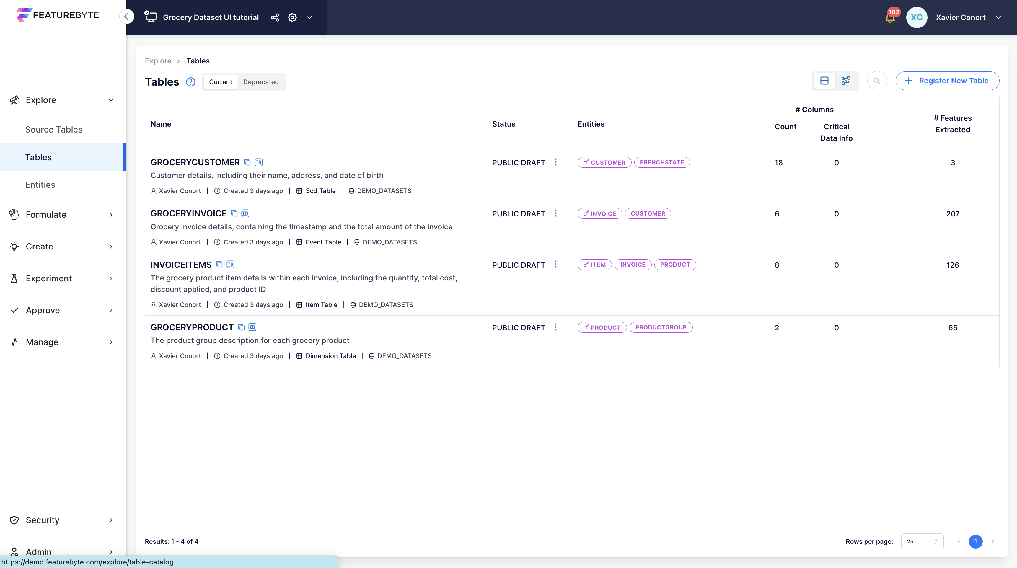
Table Catalog¶

The Tables registered in the catalog can be listed and retrieved by name for easy access and management.

SDK Reference

How to:

list tables in a catalog,
get a table from a catalog.

User Inferface

Table Catalog

Entities and Relationships¶

Entity¶

An Entity is a real-world object or concept represented or referenced by columns in your source tables.

Examples

Common examples of entities include customer, merchant, city, product, and order.

In FeatureByte, entities are used to:

identify the unit of analysis for a feature or a use case
organizing features, and feature lists in the catalog
identifying entities that can be used to serve the feature or the feature list.
establishing table relationships.

SDK Reference

Refer to the Entity object main page and how to add a new entity to a catalog.

User Interface

Learn by example with our 'Register Entities' UI tutorials.

Entity Serving Name¶

An Entity's Serving Name is the name of the unique identifier used to identify the entity during a preview or serving request. It is also the name of the column representing the entity in an observation set. Typically, the serving name for an entity is the name of the primary key (or natural key) of the table that represents the entity. An entity can have multiple serving names for convenience, but the unique identifier should remain unique.

SDK Reference

How to get the serving names of an entity.

User Interface

Learn by example with our 'Register Entities' UI tutorials.

Feature Primary Entity¶

The Primary Entity of a feature defines the level of analysis for that feature.

The Primary Entity is usually a single entity. However, there are cases where it may be a tuple of entities.

An example of when the primary entity becomes a tuple of entities is when a feature results from aggregatiing data based on those entities to measure interactions between them.

Example

Entity Diagram

Suppose a feature quantifies the interaction between a customer entity and a merchant entity in the past, such as the sum of transaction amounts grouped by customer and merchant in the past four weeks.

The primary entity of this feature is the tuple of customer and merchant.

When a feature is derived from features with different primary entities, the primary entity is determined by the entity relationships between the entities. The lowest level entity in the hierarchy is selected as the primary entity. If the entities have no relationship, the primary entity becomes a tuple of those entities.

Example

Entity Diagram

Consider two entities: customer and customer city, where the customer entity is a child of customer city entity. If a new feature is created that compares a customer's basket with the average basket of customers in the same city, the primary entity for that feature would be the customer entity. This is because the customer entity is a child of the customer city entity and the customer city entity can be deduced automatically.

Alternatively, if two entities, such as customer and merchant, do not have any relationship, the primary entity for a feature that calculates the distance between the customer location and the merchant location would be the tuple of customer and merchant entities. This is because the two entities do not have any parent-child relationship.

SDK Reference

How to get the primary entity of a feature.

Feature List Primary Entity¶

The primary entity of a feature list determines the entities that can be used to serve the feature list, which typically corresponds to the primary entity of the Use Case that the feature list was created for.

If the features within the list pertain to different primary entities, the primary entity of the feature list is selected based on the entities relationships, with the lowest level entity in the hierarchy chosen as the primary entity. In cases where there are no relationships between entities, the primary entity may become a tuple comprising those entities.

Example

Entity Diagram

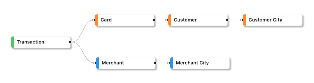
Consider a feature list containing features related to card, customer, and customer city. In this case, the primary entity is the card entity since it is a child of both the customer and customer city entities.

However, if the feature list also contains merchant and merchant city features, the primary entity is a tuple of card and merchant.

SDK Reference

How to get the primary entity of a feature list.

Serving Entity¶

A Serving Entity is any entity that can be used to preview or serve a feature or feature list, regardless of whether it is the primary entity. Serving entities associated with a feature or feature list are typically descendants of the primary entity and uniquely identify the primary entity.

Example

Entity Diagram

Suppose that a customer is the primary entity for a feature, the serving entities for that feature could include related entities such as the card and transaction entities, which are child or grandchild of the customer entity and uniquely identify the customer.

Use Case Primary Entity¶

In a Use Case, the Primary Entity is the object or concept that defines its problem statement and Context. Usually, this entity is singular, but in cases such as recommendation engines, it can be a tuple of entities such as (Customer, Product).

Observation Table Primary Entity¶

An Observation Table Primary Entity is the entity of the Context or Use Case the table represents.

To utilize an Observation Table for computing historical feature values of a feature list, it's important that its Primary Entity should match the feature list's primary entity or be a related serving entity.

Entity Relationship¶

The parent-child relationship and the supertype-subtype relationship are the two main types of Entity Relationships that can assist feature engineering and feature serving.

The parent-child relationship is automatically established in FeatureByte during the entity tagging process, while identifying supertype-subtype relationships require manual intervention.

These relationships can be used to suggest, facilitate and verify joins during feature engineering and streamline the process of serving feature lists containing multiple entity-assigned features.

Important

Note that FeatureByte only supports parent-child relationships currently. Nevertheless, it is expected that supertype-subtype relationships will also be supported shortly, thus enabling more efficient feature engineering and feature serving.

SDK Reference

Refer to the Relationship object main page or to the specific links:

list relationships between entities in a catalog.

User Interface

Learn by example with our 'Register Entities' UI tutorials.

Parent-Child Relationship¶

A Parent-Child Relationship is a hierarchical connection that links one entity (the child) to another (the parent). Each child entity key value can have only one parent entity key value, but a parent entity key value can have multiple child entity key values.

Example

Examples of parent-child relationships include:

Hierarchical organization chart: A company's employees are arranged in a hierarchy, with each employee having a manager. The employee entity represents the child, and the manager entity represents the parent.
Product catalog: In an e-commerce system, a product catalog may be categorized into categories and subcategories. Each category or subcategory represents a child of its parent category.
Geographical hierarchy: In a geographical data model, cities are arranged in states, which are arranged in countries. Each city is the child of its parent state, and each state is the child of its parent country.
Credit Card hierarchy: A credit card transaction is the child of a card and a merchant. A card is a child of a customer. A customer is a child of a customer city. And a merchant is a child of a merchant city.

Entity Diagram

Note

In FeatureByte, the parent-child relationship is automatically established when the primary key (or natural key in the context of a SCD table) identifies one entity. This entity is the child entity. Other entities that are referenced in the table are identified as parent entities.

Supertype-Subtype Relationship¶

In a data model, a Supertype-Subtype Relationship is a hierarchical relationship between two or more entity types where one entity type (the subtype) inherits attributes and relationships from another entity type (the supertype).

The subtype entity is typically a more specialized version of the supertype entity, representing a subset of the data that applies to a particular domain. Although the subtype entity inherits properties and relationships from the supertype entity, It can have its unique attributes or relationships.

Examples

Here are a few examples of supertype-subtype relationships involving a person, student, and teacher:

Person is the supertype, while student and teacher are both subtypes of person.
Student is a subtype of person. This is because a student is a specific type of person who is enrolled in a school or university.
Teacher is also a subtype of person since a teacher is a specific type responsible for educating and instructing students.
A more specific subtype of student could be a graduate student, which refers to a student who has already completed a bachelor's degree and is pursuing a higher-level degree.
Another subtype of teacher could be a professor, typically a teacher with a higher academic rank and significant experience in their field.

Supertype-subtype relationships describe how a more general category (the supertype) can be divided into more specific subcategories (the subtypes). In this case, a person is the most general category, while student and teacher are more specific categories that fall under the broader umbrella of "person."

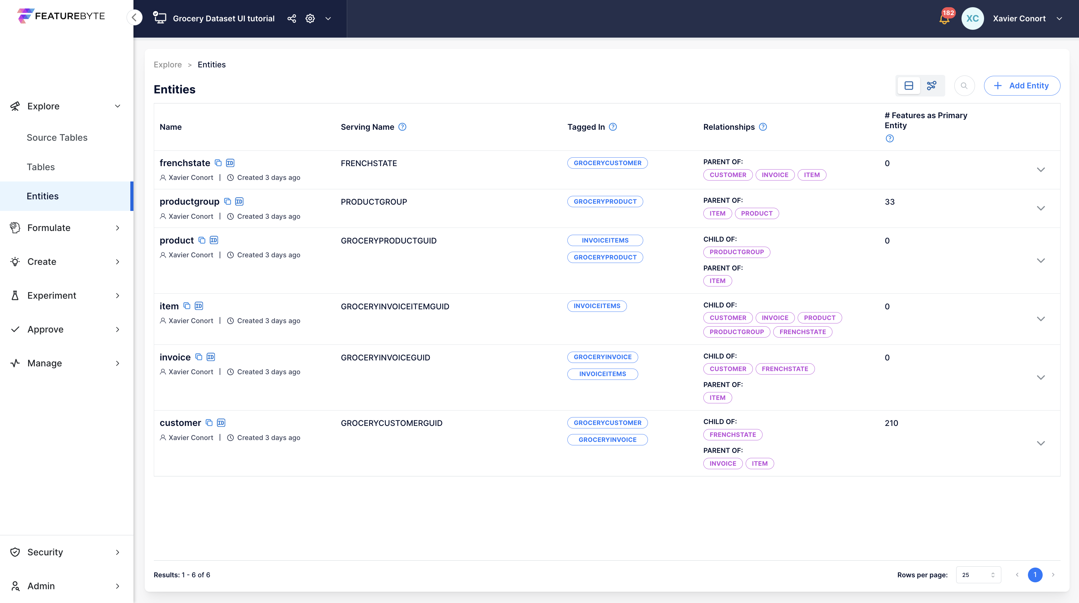
Entity Catalog¶

The Entities registered in the catalog can be listed and retrieved by name for easy access and management.

SDK Reference

How to:

list entities in a catalog,
get an entity from a catalog,

User Inferface

Entity Catalog

Use Case Formulation¶

Target¶

In Machine Learning, a "target" refers to the outcome that the model is being trained to predict. It's a critical component in supervised learning, where the goal is to create a model that can accurately forecast or classify the target based on the patterns it identifies in the input features.

In FeatureByte, a target can be established in two ways:

Descriptive Approach: You directly outline your prediction goal.
Logical Approach: This technique calculates targets within FeatureByte, mirroring the process of creating features.

SDK Reference

Refer to the Target object main page and how to create a descriptive target

User Interface

Learn by example with our 'Create Use Cases' UI tutorials.

Target Logical Plan¶

The process for establishing a logical plan for a Target closely mirrors that for creating features, with a critical difference: the plan for a Target utilizes forward operations, in contrast to the backward operations applied in feature creation.

Target objects, built upon View objects, come in three varieties:

Lookup Targets: Directly retrieve values from view attributes for a future point in time.
Forward Window-based Aggregate Targets: Use forward-looking aggregations over grouped data.
Aggregate Targets as a Future Point-in-Time: Apply aggregations at a designated future moment.

Additionally, targets can emerge as transformations of existing Target objects, offering various ways to define what you want to predict.

SDK Reference

How to:

Target Definition File¶

The target definition file is the single source of truth for a target. This file is automatically generated when a feature is declared in the SDK or a new version is derived.

The syntax used in the SDK is also used in the target definition file. The file provides an explicit outline of the intended operations of the feature declaration, including those inherited but not explicitly declared by you. These operations may include cleaning operations inherited from tables metadata.

The target definition file is the basis for generating the final logical execution graph, which is then transpiled into platform-specific SQL (e.g. SnowSQL, SparkSQL) for target materialization.

SDK Reference

How to obtain the target definition file.

User Interface

Learn by example with our 'Create Use Cases' UI tutorials.

Target Materialization¶

Materializing target values in FeatureByte using observation sets can be done through two distinct approaches:

Using compute_targets(): This method returns a DataFrame filled with target values, suitable for immediate analysis and use.
Using compute_target_table(): This approach yields an ObservationTable object, representing an observation table suitable for long-term storage and linking with a Use Case for repeated use.

SDK Reference

How to:

User Interface

Learn by example with our 'Create Observation Tables' UI tutorials.

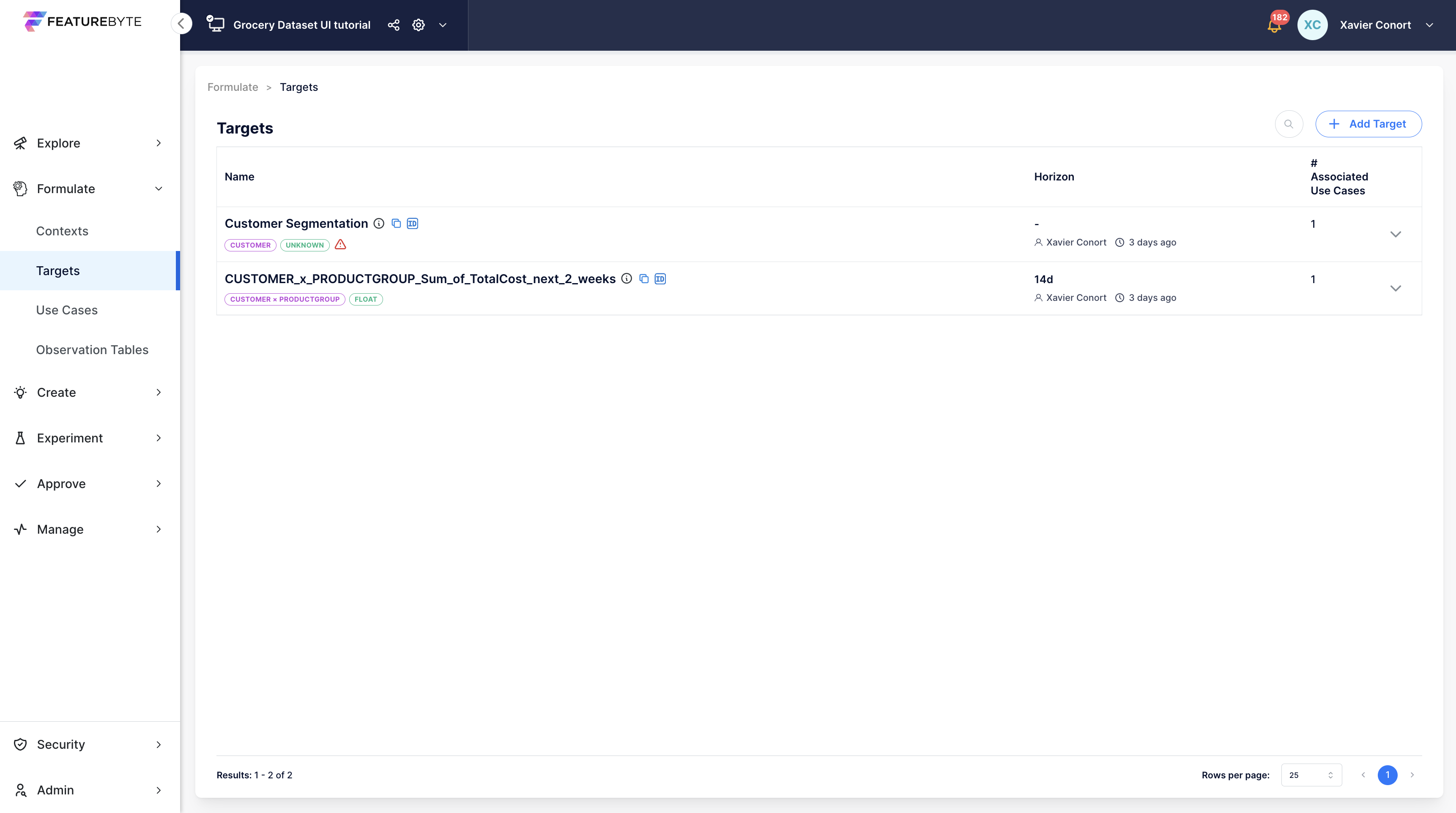
Target Catalog¶

The Targets registered in the catalog can be listed and retrieved by name for easy access and management.

SDK Reference

How to:

list targets available in a catalog
get a target from a catalog

User Inferface

How to list registered Targets.

Target Catalog

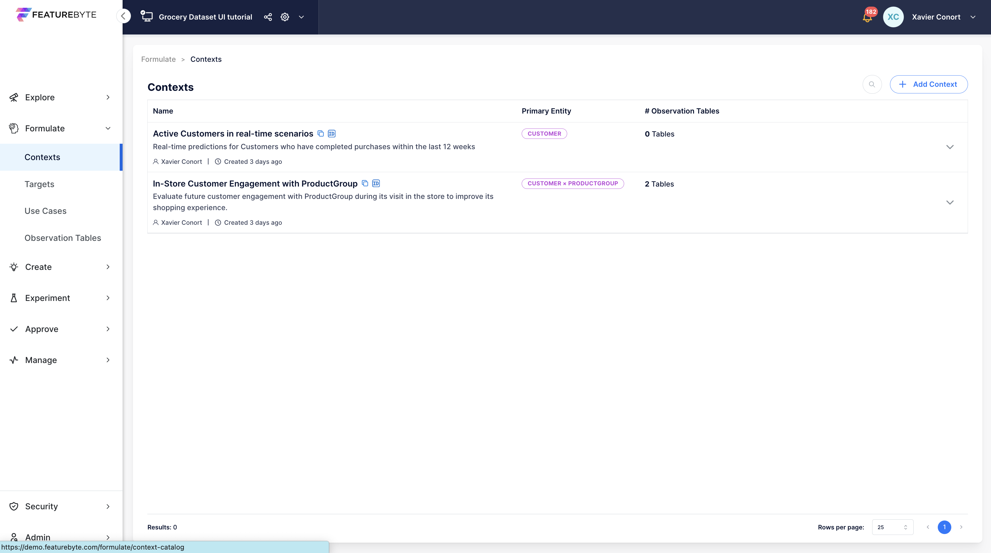
Context¶

A Context defines the scope and circumstances in which features are expected to be served.

Examples

Contexts can vary significantly. For instance:

Batch Predictions Context: Making weekly batch predictions for an active customer that has made at least one purchase over the past 12 weeks.
Real-Time Predictions Context: Offering real-time predictions for a credit card transaction that has been recently processed.

While creating a basic context requires only identifying the relevant entity, adding a detailed description is beneficial. This should ideally cover:

Contextual Subset Details: Characteristics of the entity subset being targeted.
Serving Timing: Insights into when predictions are needed, whether in batch or real-time scenarios.
Inference Data Availability: What data is available at the time of inference.
Constraints: Any legal, operational, or other constraints that might impact the context.

SDK Reference

Refer to the Context object main page and how to create a context.

User Interface

Learn by example with our 'Create Use Cases' UI tutorials.

Context Association with Observation Table¶

After defining a Context, it can be linked to an Observation Table. This process enables the observation table to act as the default preview/eda table for the Context. Additionally, all observation tables associated with the Context can be listed.

SDK Reference

How to:

User Interface

Learn by example with our 'Create Observation Tables' UI tutorials.

Context Catalog¶

The Contexts registered in the catalog can be listed and retrieved by name for easy access and management.

SDK Reference

How to:

list contexts available in a catalog
get a context from a catalog

User Inferface

How to list registered Contexts.

Context Catalog

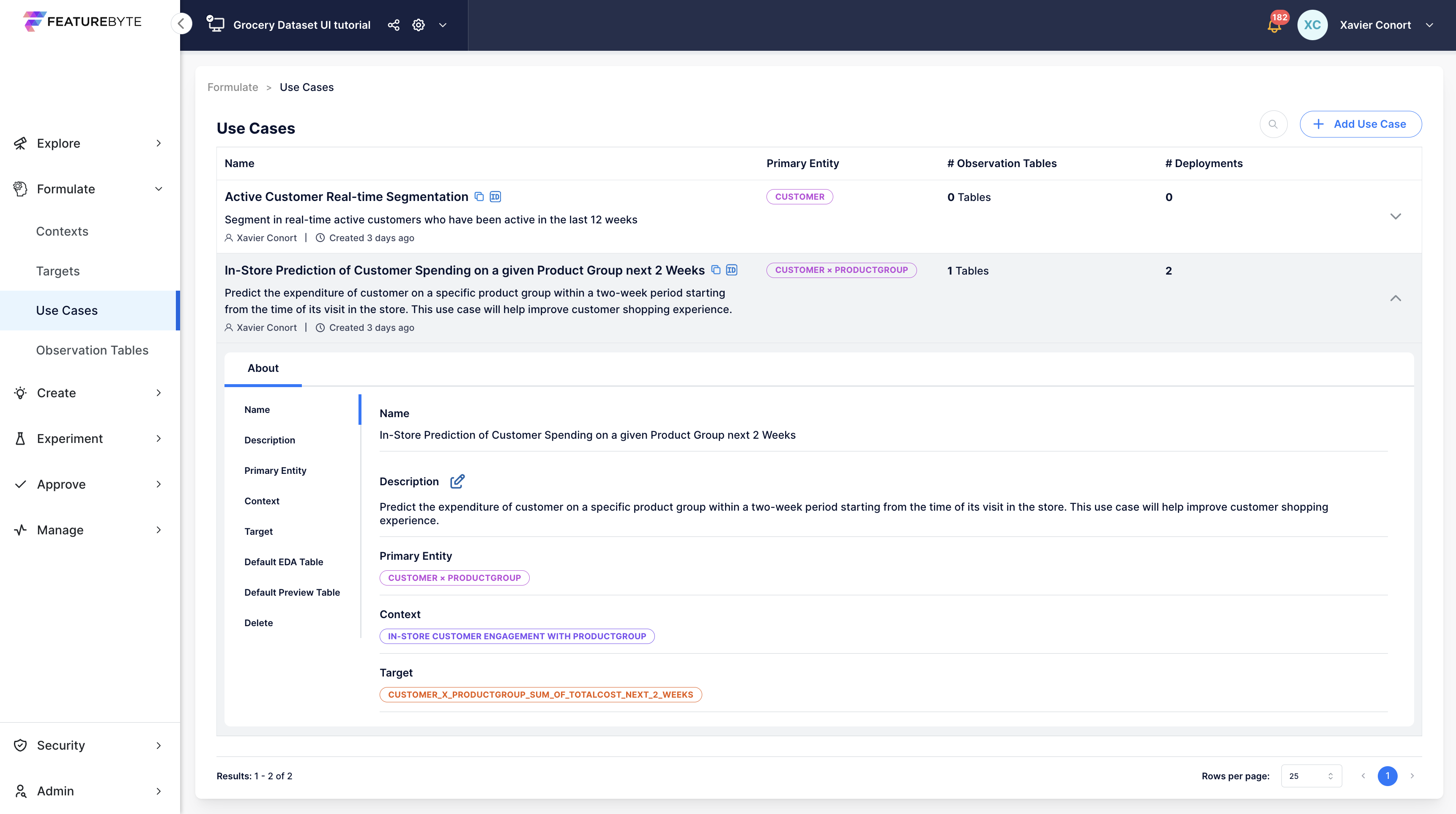
Use Case¶

A Use Case formulates the modelling problem by associating a Context with a Target. Use Cases facilitate the organization of your observation tables, feature tables and deployments. Use Cases also play a crucial role in FeatureByte Copilot, enabling it to provide tailored feature suggestions.

To construct a new Use Case, the following information is required:

Select a Context: Choose a registered Context that defines the environment of your Use Case.
Define a Target: Specify a registered Target that represents the goal of your Use Case.

Note

The context and target must correspond to the same entities.

For a comprehensive Use Case setup, include a detailed description. Providing a detailed description of the use case, context, and target ensures better documentation and enhances the effectiveness of the FeatureByte Copilot in suggesting relevant features and assessing their semantic relevance.

SDK Reference

Refer to the Use Case object main page or to the specific links:

create a use case

User Interface

Learn by example with our 'Create Use Cases' UI tutorials.

Use Case Association with Observation Table¶

Observation tables are automatically linked to a Use Case when they are derived from:

an observation table that is linked to the use case's Context
a target that is linked to the use case

An observation table can be manually linked to the Use Case to support cases where the observation table is not derived from another observation table.

This process enables the observation table to act as the default preview/eda table for the Use Case. Additionally, all observation tables associated with the Use Case can be listed.

SDK Reference

How to:

Use Case Association with Feature Table¶

Feature tables are automatically associated with use cases via the observation tables they originate from.

Feature tables associated with a use case can be listed easily from the Use Case object.

SDK Reference

How to:

Use Case Association with Deployment¶

A deployment is associated with a use case when the use case is specified during the deployment of the related feature list.

Deployments associated with a use case can be listed easily from the Use Case object.

SDK Reference

How to:

Use Case Catalog¶

The Use Cases registered in the catalog can be listed and retrieved by name for easy access and management.

SDK Reference

How to:

list use cases available in a catalog
get a use case from a catalog

User Inferface

How to list registered Use Cases.

Use Case Catalog

Observation Set¶

An Observation Set is essentially a collection of historical data points that serve as a foundation for learning. Think of it as the backbone of a training dataset. Its primary role is to process and compute features, which then form the training data for Machine Learning models. For a given use case, the same Observation Table is often employed in multiple experiments. However, the specific features chosen and the Machine Learning models applied may vary between these experiments.

Each data point represents a historical moment for a particular entity and may include target values.

Observation Set

Ideally, an observation set should be explicitly linked to a specific Context or Use Case, ensuring thorough documentation and facilitating its reuse.

Other important considerations when constructing an Observation Set are:

Choosing the Right Entity Key Values: Select values that represent your target population accurately for each historical timestamp.
Accuracy in Timestamps: Ensure all timestamps are in Coordinated Universal Time (UTC) and cover a sufficient range to depict seasonal changes. They should represent the expected time distribution in real-world scenarios.
Maintaining Data Integrity: Avoid time leakage (future data in the training set) by spacing out your timestamps correctly.

Example

To predict customer churn every Monday morning over six months, you might:

Use historical timestamps from Monday mornings of the past years
Choose customer keys randomly from the active customer base at those times.
Set intervals longer than six months between data points for each customer to avoid time leakage.

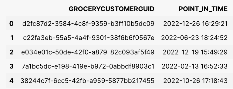
Technical Details

The entity values column should have an accepted serving name.
Label the timestamps column as "POINT_IN_TIME" and use UTC.
In FeatureByte, an Observation Set can be a pandas DataFrame or an Observation Table object from the feature store.

Once an Observation Set is defined, you can use it to materialize a feature list into historical feature values to form a training or testing set for your Machine Learning model.

SDK Reference

How to:

get the primary entity of a feature list,
compute historical feature values as a DataFrame.
compute historical feature values as a HistoricalFeatureTable object.

Observation Table¶

An Observation Table is an observation set integrated in the catalog. It can be created from various sources and is essential for sharing and reusing data within the feature store.

SDK Reference

Refer to the ObservationTable object main page or to the specific links:

User Interface

Learn by example with our 'Create Observation Tables' UI tutorials.

Observation Table Association with a Context or Use Case¶

Once added to the catalog, an Observation Table can be linked to specific Contexts or Use Cases.

For Use Case linkage, you can include the Use Case's Target values by materializing them with a table associated with its Context.

SDK Reference

How to:

Observation Table Purpose¶

Tagging an Observation Table with purposes like 'preview', 'eda', 'training' or 'validation_test' facilitates its identification and reuse.

Default eda and preview tables can also be set for a Context or a Use Case.

SDK Reference

How to:

Observation Table Catalog¶

The Observation Tables registered in the catalog can be listed and retrieved by name for easy access and management.

SDK Reference

How to:

list observation tables available in a catalog
get an observation table from a catalog
and get an observation table by its Object ID from a catalog

Views and Column Transforms¶

View¶

A view is a local virtual table that can be modified and joined to other views to prepare data before feature definition. A view does not contain any data of its own.

Views in FeatureByte allow operations similar to Pandas, such as:

creating and transforming columns and extracting lags
filtering records, capturing attribute changes, and joining views

Unlike Pandas DataFrames, which require loading all data into memory, views are materialized only when needed during previews or feature materialization.

View Creation¶

When a view is created, it inherits the metadata of the FeatureByte table it originated from. Currently, five types of views are supported:

Event Views created from an Event table
Item Views created from an Item table
Dimension Views created from a Dimension table
Slowly Changing Dimension (SCD) Views created from a SCD table
Change Views created from a SCD table.

Two view construction modes are available:

Auto (default): Automatically cleans data according to default operations specified for each column within the table and excludes special columns not meant for feature engineering.
Manual: Allows custom cleaning operations without applying default cleaning operations.

Although views provide access to cleaned data, you can still perform data manipulation using the raw data from the source table. To do this, utilize the view's raw attribute, which enables you to work directly with the unprocessed data of the source table.

SDK Reference

Refer to the View object main page or to the specific links:

Change View¶

A Change View is created from a Slowly Changing Dimension (SCD) table to provide a way to analyze changes that occur in an attribute of the natural key of the table over time. This view consists of five columns:

the natural key of the SCD table,
the change timestamp, which is equal to the effective timestamp of the SCD table,
the prior effective timestamp,
the value of the attribute before the change occurred,
and the value of the attribute after the change occurred.

Once the Change View is created, it can be used to generate features in the same way as features from an Event View.

Examples

Changes to a SCD table can provide valuable insights into customer behavior, such as:

the number of times a customer has moved in the past six months,
their previous address if they recently moved,
whether they have gone through a recent divorce,
if there are new additions to their family,
or if they have started a new job.

SDK Reference

How to create a Change View from a SCD table.

Filters¶

Filters are an essential element in feature engineering strategies. They enable the segmentation of data into sub-groups, which facilitates specific operations and analyses:

Targeted Aggregations: Filters allow for meaningful aggregations of data that would otherwise be nonsensical. For instance, transactions can be categorized by their outcomes such as "Authorized", "Approved", or "Cancelled".
Focused Analysis: By using filters, it is possible to narrow down the analysis to specific event types and derive additional, relevant features for those types. For example, analyzing transactions by weekday may yield insightful trends for "Purchases" but may be less significant for "Banking Fees".

FeatureByte Copilot leverages Generative AI to aid enterprise users in identifying effective filters.

Within our SDK, users can manipulate data similarly to how one would use a Pandas DataFrame. It is possible to create new views from subsets of views. Additionally, a condition-based subset can be used to replace the values of a column.

View Sample¶

Using the sample method, a view can be materialized with a random selection of rows for a given time range, size, and seed to control sampling.

Note

Views from tables in a Snowflake data warehouse do not support the use of seed.

SDK Reference

How to materialize a sample of a view.

View Join¶

To join two views, use the join() method of the left view and specify the right view object in the other_view parameter. The method will match rows from both views based on a shared key, which is either the primary key of the right view or the natural key if the right view is a Slowly Changing Dimension (SCD) view.

If the shared key identifies an entity that is referenced in the left view or the column name of the shared key is the same in both views, the join() method will automatically identify the column in the left view to use for the join.

By default, a left join is performed, and the resulting view will have the same number of rows as the left view. However, you can set the how parameter to 'inner' to perform an inner join. In this case, the resulting view will only contain rows where there is a match between the columns in both tables.

When the right view is an SCD view, the event timestamp of the left view determines which record of the right view to join.

Note

For Item View, the event timestamp and columns representing entities in the related event table are automatically added. Additional attributes can be joined using the join_event_table_attributes() method.

Important

Not all views can be joined to each other. SCD views cannot be joined to other SCD views, while only dimension views can be joined to other dimension views. Change views cannot be joined to any views.

SDK Reference

How to:

View Column¶

A View Column is a column within a FeatureByte view. When creating a view, a View Column represents the cleaned version of a table column. The cleaning procedure for a View Column depends on the view's construction mode and typically follows the default cleaning operations associated with the corresponding table column.

By default, special columns not intended for feature engineering are excluded from view columns. These columns may consist of record creation and expiration timestamps, surrogate keys, and active flags.

You can add new columns to a view by performing joins or by deriving new columns from existing ones.

If you wish to add new columns derived from the raw data in the source table, use the view's raw attribute to access the source table's unprocessed data.

SDK Reference

Refer to the ViewColumn object main page or to the specific links:

obtain view columns info
access raw data
and obtain descriptive statistics for a view column.

View Column Transforms¶

View Column Transforms refer to the ability to apply transformation operations on columns within a view. By applying these transformation operations, you can create a new column. This new column can either be reassigned to the original view or utilized for further transformations.

The different types of transforms include:

generic transforms,
numeric transforms,
string transforms,
datetime transforms,
and lag transforms.

Additionally, you have the option to apply custom SQL User-Defined Functions (UDFs) on view columns. This is particularly useful for integrating transformer models with FeatureByte.

Generic Transforms¶

SDK Reference

You can apply the following transforms to columns of any data type in a view:

isnull: Returns a new boolean column that indicates whether each row is missing.
notnull: Returns a new boolean column that indicates whether each row is not missing.
isin: Returns a new boolean column showing whether each element in the view column matches an element in the passed sequence of values
fillna: Replaces missing values in-place with specified values.
astype: Converts the data type of the column.

Numeric Transforms¶

SDK Reference

In addition to built-in arithmetic operators (+, -, *, /, etc), you can apply the following transforms to columns of numeric type in a view:

abs: Returns absolute value
sqrt: Returns square root value
pow: Returns power value
log: Returns logarithm with natural base
exp: Returns exponential value
floor: Rounds down to the nearest integer
ceil: Rounds up to the nearest integer

String Transforms¶

API Reference

In addition to string columns concatenation, you can apply the following transforms to columns of string type in a view:

len: Returns the length of the string
lower: Converts all characters to lowercase
upper: Converts all characters to uppercase
strip: Trims white space(s) or a specific character on the left & right string boundaries
lstrip: Trims white space(s) or a specific character on the left string boundaries
rstrip: Trims white space(s) or a specific character on the right string boundaries
replace: Replaces substring with a new string
pad: Pads string up to the specified width size
contains: Returns a boolean flag column indicating whether each string element contains a target string
slice: Slices substrings for each string element

Datetime Transforms¶

The date or timestamp (datetime) columns in a view can undergo the following transformations:

Calculate the difference between two datetime columns.
Add a time interval to a datetime column to generate a new datetime column.
Extract date components from a datetime column.

Note

Date parts for columns or features using timestamp with time zone offset are based on the local time instead of UTC.

Date parts for columns or features using event timestamps of Event tables, where a separate column was specified to provide the time zone offset information, will also be based on the local time instead of UTC.

SDK Reference

How to extract date components:

microsecond: Returns the microsecond component of each element
millisecond: Returns the millisecond component of each element
second: Returns the second component of each element
minute: Returns the minute component of each element
hour: Returns the hour component of each element
day: Returns the day component of each element in a view column
day_of_week: Returns the day of week component of each element
week: Returns the week component of each element
month: Returns the month component of each element
quarter: Returns the quarter component of each element
year: Returns the year component of each element

Lag Transforms¶

The use of Lag Transforms enables the retrieval of the preceding value associated with a particular entity in a view.

This, in turn, makes it feasible to compute essential features, such as those that depend on inter-event time and the proximity to the previous point.

Note

Lag transforms are only supported for Event and Change views.

SDK Reference

How to extract lags from a view column.

UDF Transforms¶

A SQL User-Defined Function (UDF) is a custom function created by users to execute specific operations not covered by standard SQL functions. UDFs encapsulate complex logic into a single, callable routine.

An application of this is in computing text embeddings using transformer-based models or large language models (LLMs), which can be formulated as a UDF.

Creating a SQL Embedding UDF

For step-by-step guidance on creating a SQL Embedding UDF, visit the Bring Your Own Transformer tutorials.

SDK Reference

Refer to the UserDefinedFunction object main page or to the specific links:

make the function available to the FeatureByte SDK,
retrieve a UDF instance from the catalog,

Feature Creation¶

Features¶

Input data used to train Machine Learning models and compute predictions is referred to as features.

These features can sometimes be derived from attributes already present in the source tables.

Example

A customer churn model may use features obtained directly from a customer profile table, such as age, gender, income, and location.

However, in many cases, features are created by applying a series of row transformations, joins, filters, and aggregates.

Example

A customer churn model may utilize aggregate features that reflect the customer's account details over a given period, such as

the customer entropy of product types purchased over the past 12 weeks,
the customer count of canceled orders over the past 56 weeks,
and the customer amount spent over the past seven days.

FeatureByte offers two ways to create features:

Manually: Using the SDK declarative framework
Automatically: Using FeatureByte Copilot

Feature Object¶

A Feature object in FeatureByte SDK contains the logical plan to compute the feature.

There are three ways to define the plan for Feature objects from views:

Lookup features
Aggregate features
Cross Aggregate features

Additionally, Feature objects can be created as transformations of one or more existing features.

SDK Reference

Refer to the Feature object main page or to the specific links:

create a Lookup feature,
and group by entity for Aggregates and Cross Aggregates.

Lookup Features¶

A Lookup Feature refers to an entity’s attribute in a view at a specific point-in-time. Lookup features are the simpler form of a feature as they do not involve any aggregation operations.

When a view's primary key identifies an entity, it is simple to designate its attributes as features for that particular entity.

Examples

Examples of Lookup features are a customer's birthplace retrieved from a Customer Dimension table or a transaction amount retrieved from a Transactions Event table.

When an entity serves as the natural key of an SCD view, it is also possible to assign one of its attributes as a feature for that entity. However, in those cases, the feature is materialized through point-in-time joins, and the resulting value corresponds to the active row at the point-in-time specified in the feature request.

Example

A customer feature could be the customer's street address at the request's point-in-time.

When dealing with an SCD view, you can specify an offset if you want to get the feature value at a specific time before the request's point-in-time.

Example

By setting the offset to 9 weeks in the previous example, the feature value would be the customer's street address nine weeks before the request's point-in-time.

SDK Reference

How to create a Lookup feature.

Aggregate Features¶

Aggregate features are a fundamental aspect of feature engineering, essential for transforming transactional data into meaningful insights. These features are derived by applying a range of aggregation functions to data points grouped by one or more entities.

Supported aggregation functions include:

Latest: This function retrieves the most recent value in a column for an entity. It's particularly useful for datasets where the latest information is of prime importance, such as in tracking recent user activity.
Count Counts the number of occurrences for an entity. Useful in scenarios requiring a count of events or items, like the number of transactions per customer or the frequency of specific events.
NA Count Tallies the number of missing data points in a column for an entity. This is particularly valuable in datasets where the presence of missing data can indicate significant trends or issues.
Sum: Calculates the total sum of a colum values for an entity. This function is essential in aggregating numerical data, such as totaling expenditures per customer or aggregating resource usage.
Average (Mean): Computes the mean value of column values for an entity. This function is key in finding the average or typical value, applicable in various contexts like calculating the average spending of customers or the average temperature over a period. It is also applicable in computing the mean vector of embeddings in multi-dimensional data spaces, useful in fields like natural language processing or image analysis.
Minimum and Maximum: Identifies the lowest and highest values in a column for an entity, respectively. They are essential for understanding the range of data, such as the minimum and maximum temperatures recorded. The Maximum function is particularly useful in text embeddings to highlight the most significant features in text data.
Standard Deviation: Calculates the measure of variability or dispersion around the mean of column values for an entity. It's significant in assessing the spread or distribution of data points.

SDK Reference

How to access the list of aggregation methods.

While leveraging these aggregation functions, it's crucial to incorporate the temporal dimension of the dataset to ensure meaningful and contextually relevant aggregations. Ignoring the temporal dimension would also lead to temporal leakage.

There are three main types of aggregate features:

Non-Temporal Aggregates,
Aggregates Over a Window
and Aggregates "As At" a Point-in-Time.

Note

If a feature is intended to capture patterns of interaction between two or more entities, these aggregations are grouped by the tuple of the entities. For instance, an aggregate feature can be created to show the amount spent by a customer with a merchant in the past.

SDK Reference

How to create:

a non-temporal aggregate feature,
an aggregate over feature,
an aggregate "asat" feature.

Cross Aggregate Features¶

Cross Aggregate Features in FeatureByte provide a powerful mechanism to aggregate data across categorical columns, enabling sophisticated data analysis and insight generation. This functionality allows you to categorize data into groups (a process known as 'bucketing') based on categorical column values and perform various aggregation operations like counting records within each category or summing up values of a numeric column for those categories. Beyond counting and summing, you can employ additional aggregation methods tailored to your analysis needs.

This feature facilitates advanced analytical tasks, such as:

Entropy Analysis: This involves assessing the entropy in data distributions that emerge from aggregating sums or counts across categories. Such analysis is crucial for understanding data variability or diversity, shedding light on the unpredictability in aspects like customer behavior or product performance.
Temporal and Comparative Distribution Analysis: This feature enables the comparison of category-based distributions over time or against overarching groups. It's instrumental in tracking how engagements within categories evolve over time or in relation to larger entities.
Identifying Key Categories: This aspect focuses on uncovering significant trends or preferences within your data. It includes:
- Identifying the most frequently occurring category, highlighting prevalent trends.
- Pinpointing categories with the highest or lowest aggregated values, such as sales or user engagement, to recognize outstanding or lagging areas.
- Aggregating values for a specific category to gain detailed insights into particular segments of interest.
Prevalence of Entity Attributes: This involves a multi-step process to evaluate the commonality of certain attributes within entities, such as assessing customer age bands across products. Steps might include aggregating by product across age bands, followed by a comprehensive aggregation across these bands, and then analyzing proportions to understand demographic affinities or discrepancies for specific products.

Example Use Case

Imagine analyzing customer spending habits. A Cross Aggregate feature might calculate the total amount spent by each customer across different product categories over a specified period. This aggregation offers insights into customer spending patterns or preferences, enriching understanding of behavior across various product categories.

Technical Implementation

When computing Cross Aggregate features for an entity (e.g., a customer), the outcome is typically structured as a dictionary. This dictionary's keys are the product categories engaged by the customer, with values representing total expenditure in each category. This structure effectively captures the customer's cross-category spending behavior, providing a holistic view of their purchase preferences.

Like other types of Aggregate Features, it is important to consider the temporal aspect when conducting aggregation operations. The three main types of Cross Aggregate features include:

Non-Temporal Cross Aggregate,
Cross Aggregate Over a Window
Cross Aggregate "As At" a Point-in-Time.

SDK Reference

How to group by entity across categories to perform cross aggregates.

Non-Temporal Aggregates¶

Non-Temporal Aggregate features refer to features that are generated through aggregation operations without considering any temporal aspects. In other words, these features are created by aggregating values without considering the order or sequence in which they occur.

Important

To avoid time leakage, the non-temporal aggregate is only supported for Item views, when the grouping key is the event key of the Item view. An example of such features is the count of items in Order.

Note

Non-temporal aggregate features obtained from an Item view can be added as a column to the corresponding event view. Once the feature is integrated, it can be aggregated over a time window to create aggregate features over a window. For instance, you can calculate a customer's average order size over the last three weeks by using the order size feature extracted from the Order Items view and aggregating it over that time frame in the related Order view.

SDK Reference

How to:

create a non-temporal aggregate feature,
and add a feature as a column.

Aggregates Over A Window¶

Aggregates over a window refer to features generated by aggregating data within a specific time frame. These types of features are commonly used for analyzing event and item data.

The duration of the window is specified when the feature is created. The end point of the window is determined when the feature is served, based on the point-in-time values specified by the feature request and the feature job setting of the feature.

SDK Reference

How to create an aggregate over feature.

Aggregates “As At” a Point-In-Time¶

Aggregates "As At" a Point-In-Time are features that are generated by aggregating data that is active at a particular moment in time. These types of features are only available for slowly changing dimension (SCD) views and the grouping key used for generating these features should not be the natural key of the SCD view.

You can specify an offset, if you want the aggregation to be done on rows active at a specific time before the point-in-time specified by the feature request.

Example

An aggregate ‘as at’ feature from a Credit Cards table could be the customer's count of credit cards at the specified point-in-time of the feature request.

With an offset of 2 weeks, the feature would be the customer's count of credit cards 2 weeks before the specified point-in-time of the feature request.

SDK Reference

How to create an aggregate "asat" feature.

Aggregates Of Changes Over a Window¶

Aggregates of changes over a window are features that summarize changes in a Slowly Changing Dimension (SCD) table within a specific time frame. These features are created by aggregating data from a Change view that is derived from a column in the SCD table.

Example

One possible aggregate feature of changes over a window could be the count of address changes that occurred within the last 12 weeks for a customer.

SDK Reference

How to create:

a change view from a SCD table.
and an aggregate over feature from a change view.

Temporal Window¶

In feature engineering, a "Temporal Window" refers to a specific period over which data points are gathered and analyzed to extract valuable features for modeling. Employing multiple windows enables the capture of dynamics across short, medium, and long-term intervals within the data.

Window Size determines the duration of the temporal window (e.g., minutes, hours, days, weeks), and its selection depends on the specific use case and data characteristics.

FeatureByte Copilot assists enterprise users in identifying the most appropriate window sizes for their particular applications.

Examples

Shop Sum of sales over the past 4 weeks.
Total call duration by a customer over the week.
Rolling average of heart rate variability over the last 24 hours.
Maximum machine temperature recorded in the last 30 minutes.

Edge Effects

At the Beginning of the Data: Ensure the starting point of your training data is after the initial table observations plus the window size. This adjustment prevents incomplete data windows at the start of the dataset.
At the End of the Data: Set a sufficiently large blind spot in the feature job settings to account for the potential unavailability of the most recent data points due to data latency.

Feature Transforms¶

Feature Transforms is a flexible functionality that allows the generation of new features by applying a broad range of transformation operations to existing features. These transformations can be applied to individual features or multiple features from the same or distinct entities.

The available transformation operations resemble those provided for view columns. However, additional transformations are also supported for features resulting from Cross Aggregate features.

Features can also be derived from multiple features and the points-in-time provided during feature materialization.

Examples of features derived from Cross Aggregates

Most common weekday for customer visits in the past 12 week
Count of unique items purchased by a customer in the past 4 weeks
List of distinct items bought by a customer in the past 4 weeks
Amount spent by a customer on ice cream in the past 4 weeks
Weekday entropy for customer visits in the past 12 weeks

Examples of features derived from multiple features

Similarity between customer’s basket during the past week and past 12 weeks
Similarity between a customer's item basket and the baskets of customers in the same city over the past 2 weeks
Order amount z-score based on a customer's order history over the past 12 weeks

SDK Reference

How to transform the dictionary output of cross aggregate features:

get_value: Retrieves the value based on the key provided.
most_frequent: Retrieves the most frequent key.
unique_count: Computes number of distinct keys.
entropy: Computes the entropy over the keys.
get_rank: Computes the rank of a particular key.
get_relative_frequency: Computes the relative frequency of a particular key.
cosine_similarity: Computes the cosine similarity with another cross aggregate feature.

FeatureByte Copilot¶

FeatureByte Copilot is an AI-powered tool designed to enhance the process of feature creation.

Key Features¶

Identifying Relevant Data¶

Data Location: Finds relevant tables and entities for specific use cases.
Semantic Tagging: Employs Generative AI to tag data columns without semantic tags, aligning with a specialized ontology for feature engineering.

Feature Engineering Recommendations¶

Time Window Recommendation: Suggests specific time windows for data aggregation based on the use case.
Data Filtering Guidance: Provides advice on data filtering while considering various event types and their statuses.
Identification of Key Numeric Aggregation Column: Recommends for each table a numeric column for constructing aggregated features across categories allowing advanced feature engineering and complement features that would solely rely on counts.

Automatic Feature Proposal¶

Feature Proposals: Automatically proposes features post-establishment of data semantics, time periods, and filters, adhering to feature engineering best practices.

Feature Evaluation and Compilation¶

Relevance Evaluation: Uses Generative AI to assess the relevance of features to the intended use case.
Redundancy Check: Cross-references with existing features to prevent feature redundancy.

Feature Integration Methods¶

Direct Catalog Addition: Offers a no-code interface for straightforward integration into the Catalog.
Notebook Download Option: Allows downloading notebooks for detailed examination and customization.

User Interface

See FeatureByte in action in our UI tutorials: Discover and Create Features with FeatureByte Copilot.

For more in-depth information, refer to our White Paper on FeatureByte Copilot.

Feature Catalog¶

The Features registered in the catalog can be listed and retrieved by name for easy access and management.

In the SDK, features can be filtered based on two key attributes:

Primary Entity
and Primary Table.

SDK Reference

list features in a catalog,
get a feature from a catalog,

Self-Organized Feature Catalog¶

FeatureByte Enterprise enhances the Feature Catalog with advanced capabilities:

Use Case Compatibility: It ensures that only features compatible with a defined Use Case are displayed, as detailed in Feature Compatibility with a Use Case.
Signal Type Categorization: Features are categorized by their Signal Type, facilitating easier identification and use.
Thematic Organization: Features are organized thematically, incorporating three key aspects:
- The feature's Primary Entity
- The feature's Primary Table
- The feature's Signal Type

In addition to basic filters, advanced filtering options in FeatureByte Enterprise include:

Signal Type.
Online Status.
Production readiness.
Feature data types.

User Interface

Learn by example with our 'Create Feature List' UI tutorials.

Feature Compatibility with a Use Case¶

In the context of a Use Case, it's crucial to ensure that the features are compatible with the Use Case Primary Entity . For a feature to be considered compatible, its Primary Entity must align with the Use Case Primary Entity in one of two ways:

Direct Match: The feature's Primary Entity should be the same as the Use Case Primary Entity.
Hierarchical Relationship: The feature's Primary Entity should be either a parent or grandparent of the Use Case Primary Entity.

Example

Entity Diagram

Consider the following scenario:

Use Case: Card Default Prediction. Use Case Primary Entity: Card.

Feature in Question: A feature that records the maximum distance between a customer's residence and the locations of their card transactions over the past 24 hours. Feature Primary Entity: Customer.

Analysis: This feature is compatible with the Use Case. Despite the Feature Primary Entity being 'Customer', it is directly linked to the 'Card' entity, which uniquely identifies each customer. Therefore, the feature can be effectively utilized in the Card Default Prediction Use Case.

In FeatureByte Enterprise, this concept plays a crucial role by ensuring that only features compatible with a defined Use Case are displayed in the Feature Catalog. This functionality streamlines the selection process and enhances the overall effectiveness of Use Case implementation.

Feature Signal Type¶

In FeatureByte, the 'signal type' of a feature is a key indicator of the information it captures. This categorization is essential not only during feature ideation but also in organizing features in the catalog and assessing the comprehensiveness of a feature list.

Signal Type Examples

Attribute: gets the attribute of the entity at a point-in-time. For instance, it might record the employment status of a customer at a specific time.
Frequency: counts the occurrence of events, like the number of times a user logs into an application.
Recency: measures the time since the latest event, crucial in tracking customer engagement.
Timing: relates to when the events happened, helpful in understanding the regularity of events such as binge watching.
Latest event: attributes of the latest event, such as the latest transaction location in a credit card record.
Stats: aggregates a numeric column's values, like the total spent by a customer over the past 4 weeks.
Diversity: measures the variability of data values, useful in understanding the range of customer preferences.
Stability: compares recent events to those of earlier periods to gauge consistency.
Similarity: compares an individual entity feature to a group, important in anomaly detection.
Most frequent: gets the most frequent value of a categorical column, like the best-selling product in a store.
Bucketing: aggregates a column's values across categories of a categorical column, allowing multi-dimensional analysis.
Attribute stats: collects stats for an attribute of the entity, such as the representation of a customer age in the overall population purchases.
Attribute change: measures the occurrence or magnitude of changes to slowly changing attributes, crucial to detect key changes in the customer environment.

Tutorials

See examples of features categorized by their signal type in the 'Learn by examples' SDK tutorial or our 'Create Feature List' UI tutorials.

Automated Signal Type tagging¶

FeatureByte Enterprise simplifies the categorization of features by their signal types through an automated tagging system. This intelligent system ensures each feature is accurately and consistently associated with its relevant signal type, reducing manual effort and enhancing the efficiency of the cataloging process.

Feature Primary Table¶

The Feature Primary Table is the central table, serving as the foundational source of data for the feature.

In a setup where an SCD table is joined with an Event table, the event table typically acts as the primary table. It contains the main events or transactions of interest, and these events are further enriched by joining with the SCD table.

Feature Secondary Table¶

The Feature Secondary Table supplements the primary table by providing additional attributes or dimensions. This table is typically joined with the primary table to enhance the data with more context.

Feature Theme¶

The Feature Theme is a concept in FeatureByte Enterprise, utilized to systematically categorize and organize features within the feature catalog. This categorization is achieved by integrating three key components:

Primary Entity: This element represents the main focus of the feature. It's the central aspect around which the feature is built.
Primary Table: This is the core database table from which the feature primarily draws its data. It provides the foundational dataset that defines the structure and context of the feature.
Signal Type: This component identifies the nature of the data signals used in the feature.

This thematic organization aids in providing a clear and structured view of the feature catalog, facilitating easier navigation and understanding of the available features.

Feature Relevance¶

Feature relevance is essential for evaluating the impact of individual features on predictive models before modeling. Two key metrics are utilized to assess feature relevance:

Predictive Score¶

The Predictive Score (PS) measures the relationship between a feature and the target variable within a specific use case. A PS score of 1 indicates perfect correlation with the target, while 0 suggests no correlation.

Note

PS evaluates features independently and might overlook potential interactions among them, which could significantly affect predictive relevance. Some features may exhibit limited predictive utility when analyzed alone. However, when combined with others, they might reveal significant predictive power due to interaction effects.

Details

PS utilizes specialized models such as XGBoost for numerical, categorical, or dictionary features, and regularized linear regression for textual features. Evaluation involves fundamental statistical measures:

For regression, it's represented as R², indicating the proportion of the variance in the target variable that is predictable from the feature.
In classification, it's calculated as 2x(AUC - 0.5), where AUC is the Area Under the ROC Curve, providing a measure of the model's ability to discriminate between positive and negative classes.

Semantic Relevance¶

Semantic relevance, derived through Generative AI, examines the significance of each feature within a specific use case based on its semantic value without directly analyzing the data. This metric considers both the feature's description and the context of the use case. It complements the predictive score by ensuring that features not only display statistical correlation with the target variable but also carry contextual meaning.

High semantic relevance scores, combined with low statistical correlation, may indicate potential data quality issues or highlight the limitations of relying solely on statistical relevance. Semantic relevance can also capture critical constraints such as fairness, causality, and other contextual factors.

Feature Materialization¶

The act of computing the feature is known as Feature Materialization.

The materialization of features is made:

on demand to fulfill historical requests,
whereas for prediction purposes, feature values are pre-computed through a batch process called a "Feature Job".

The Feature Job is scheduled based on the defined settings associated with each feature.

To materialize the feature values, either:

entities to which the feature is assigned
or their descendant entities (the serving entities) must be instantiated.

Additionally, in the context of historical feature serving, an observation set is required, created by combining:

entity key values
and point-in-time references that correspond to particular moments in the past.

Point-In-Time¶

A Point-In-Time for a feature refers to a specific moment in the past with which the feature's values are associated.

It is a crucial aspect of historical feature serving that allows Machine Learning models to make predictions based on historical data. By providing a point-in-time, a feature can be used to train and test models on past data, enabling them to make accurate predictions for similar situations in the future.

Feature Governance¶

Feature Version¶

A Feature Version enables the reuse of a Feature with varying feature job settings or distinct cleaning operations.

If the availability or freshness of the source table change, new versions of the feature can be generated with a new feature job setting. On the other hand, if changes occur in the data quality of the source table, new versions of the feature can be created with new cleaning operations that address the new quality issues.

To ensure the seamless inference of Machine Learning tasks that depend on the feature, old versions of the feature can still be served without any disruption.

Note

In the FeatureByte SDK, a new feature version is a new Feature object with the same namespace as the original Feature object. The new Feature object has its own Object ID and version name.

SDK Reference

How to:

create a new feature version,
list versions for a feature,
get the feature version name,
get the feature version Object ID,
get a specific version for a feature from a catalog,
get a specific version by its Object ID from a catalog,
and set default version

Feature Readiness¶

To help differentiate features that are in the prototype stage and features that are ready for production, a feature version can have one of four readiness levels:

PRODUCTION_READY: ready for deployment in production environments.
PUBLIC_DRAFT: shared for feedback purposes.
DRAFT: in the prototype stage.
DEPRECATED: not advised for use in either training or prediction.

Important

Only one feature version can be designated as PRODUCTION_READY at a time.

When a feature version is promoted to PRODUCTION_READY, guardrails are applied automatically to ensure consistency with defauft cleaning operations and feature job settings. You can disregard these guardrails if the settings of the promoted feature version adhere to equally robust practices.

Important Note for FeatureByte Enterprise Users

In Catalogs with Approval Flow enabled, moving features to production-ready status involves a comprehensive approval process.

This includes several evaluations, such as checking the feature's compliance with default cleaning operations and the feature job setting of its source tables. It also involves confirming the status of these tables and backtesting the feature job setting to prevent future training-serving inconsistencies. Additionally, essential details of the feature, particularly its feature definition file, are shared and subjected to a thorough review.

SDK Reference

How to:

change readiness of a feature version.

User Interface

Learn by example with our 'Deploy and serve a feature list' UI tutorials.

Default Feature Version¶

The default version of a feature streamlines the process of reusing features by providing the most appropriate version. Additionally, it simplifies the creation of new versions of feature lists.

By default, the feature's version with the highest level of readiness is considered, unless you override this selection. In cases where multiple versions share the highest level of readiness, the most recent version is automatically chosen as the default.

Note

When a feature is accessed from a catalog without specifying its object ID or its version name but only by its name, the default version is automatically retrieved.

SDK Reference

How to:

Feature Definition File¶

The feature definition file is the single source of truth for a feature version. This file is automatically generated when a feature is declared in the SDK or a new version is derived.

The syntax used in the SDK is also used in the feature definition file. The file provides an explicit outline of the intended operations of the feature declaration, including those inherited but not explicitly declared by you. For example, these operations may include feature job settings and cleaning operations inherited from tables metadata.

The feature definition file is the basis for generating the final logical execution graph, which is then transpiled into platform-specific SQL (e.g. SnowSQL, SparkSQL) for feature materialization.

Definition File

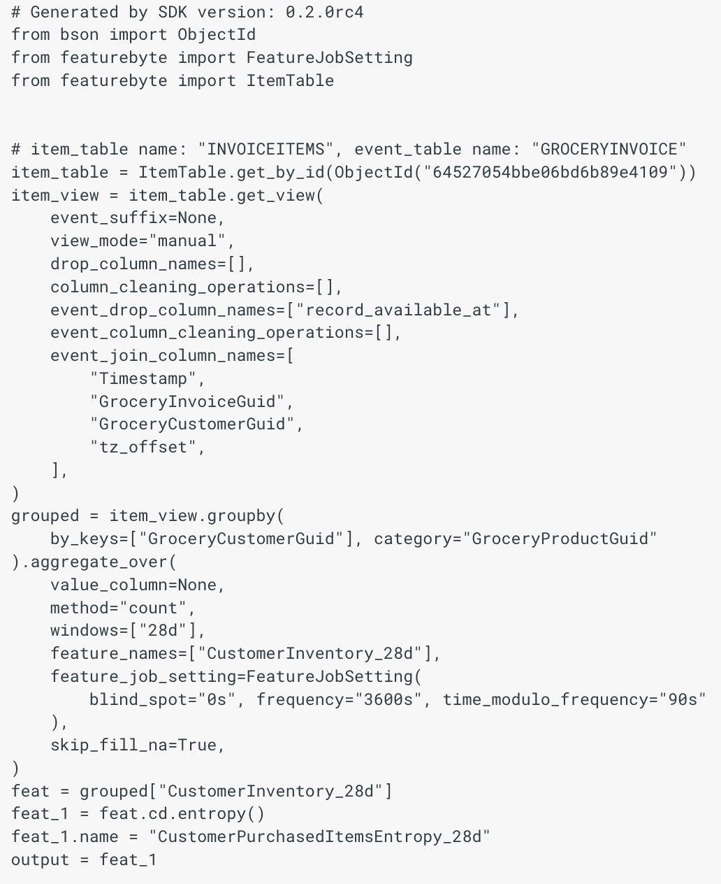
SDK Reference

How to obtain the feature definition file.

Feature Online Enabled¶

An online enabled feature is a feature that is used by at least one deployed feature list.

SDK Reference

How to obtain the feature online-enabled property.

Feature List Creation¶

Feature List¶

A Feature List is a collection of features. It is usually tailored to meet the needs of a particular use case and generate feature values for Machine Learning training and inference.

Historical feature values are first obtained to train and test models.

Once a model has been trained and validated, the Feature List can be deployed, and pre-computed feature values can be stored in the feature store and accessed through online and batch serving to generate predictions.

SDK Reference

Refer to the FeatureList object main page or to the specific links:

create a feature list,
list features in a feature list.

User Interface

Learn by example with our 'Create Feature List' UI tutorials.

Feature Group¶

A Feature Group is a temporary collection of features that facilitates the manipulation of features and the creation of feature lists.

Note

It is not possible to save the Feature Group as a whole. Instead, each feature within the group can be saved individually. To save a Feature Group as whole, convert it first as a Feature List.

SDK Reference

Refer to the FeatureGroup object main page or to the specific links:

Feature List Builder¶

The Feature List Builder is the User Interface version of a Feature Group in FeatureByte Enterprise to facilitate the construction of new feature lists. It becomes active once a specific Use Case is identified. Users can then enrich their feature list by selecting relevant features from two resources: the Feature Catalog or the Feature List Catalog.

This tool offers real-time statistics on several aspects: the readiness level of the selected features, which indicates the percentage of features that are production ready, the percentage of features currently active online, and the diversity of themes incorporated into the list.

Moreover, it dynamically suggests additional features from unrepresented themes. This recommendation system is designed to ensure the feature list encompasses a broad spectrum of signals, enhancing the overall predictive power of the feature list.

User Interface

Learn by example with our 'Create Feature List' UI tutorials.

Feature List Catalog¶

The Feature Lists registered in the catalog can be listed and retrieved by name for easy access and management.

SDK Reference

How to:

list feature lists in a catalog,
get a feature list from a catalog,

In the SDK, feature lists can be filtered based on three key attributes:

The Primary Entity of the Feature List
The Primary Tables used by the features within the lists.
The Primary Entities used by the features within the lists.

In FeatureByte Enterprise, feature lists can also be filtered based on:

Use Case, as detailed in Feature List Compatibility with a Use Case
Usage Status.
Production readiness.
Percentage of features deployed in production.
Exclusion of lists containing certain feature data types

Feature List Compatibility with a Use Case¶

In the context of a Use Case, it's crucial to ensure that the feature lists are compatible with the Use Case Primary Entity. For a feature list to be considered compatible, its Primary Entity must align with the Use Case Primary Entity in one of two ways:

Direct Match: The feature list's Primary Entity should be the same as the Use Case Primary Entity.
Hierarchical Relationship: The feature list's Primary Entity should be either a parent or grandparent of the Use Case Primary Entity.

In FeatureByte Enterprise, this concept plays a crucial role by ensuring that only feature lists compatible with a defined Use Case are displayed in the Feature List Catalog User Interface.

Example

Entity Diagram

Consider the following scenario:

Use Case: Card Default Prediction. Use Case Primary Entity: Card.

Feature List in Question: The feature list contains 2 features. - A feature that records the maximum distance between a customer's residence and the locations of their card transactions over the past 24 hours. - A feature on the Customer City population. The Feature List Primary Entity: Customer.

Analysis: This feature list is compatible with the Use Case. Despite the Feature List Primary Entity being 'Customer', it is directly linked to the 'Card' entity, which uniquely identifies each customer. Therefore, the feature can be effectively utilized in the Card Default Prediction Use Case.

Feature List Thematic Coverage¶

FeatureByte Enterprise leverages the systematic thematic categorization of features by analysing the Feature Theme attributed to each feature in a given feature list to assess its comprehensiveness. Any thematic areas that are not adequately covered by the existing features in the list are highligthed as "Themes not covered".

Feature List Serving¶

Note

A feature list can be served by its primary entity or any descendant serving entities.

Historical Feature Serving¶

Historical serving of a feature list is usually intended for exploration, model training, and testing. The requested data is represented by an observation set that combines entity key values and historical points-in-time, for which you want to materialize feature values.

Requesting historical features is supported by two methods:

compute_historical_features(): returns a loaded DataFrame. Use this method when the output is expected to be of a manageable size that can be handled locally.
compute_historical_feature_table(): returns a HistoricalFeatureTable object representing the output table stored in the feature store. This method is suitable for handling large tables and storing them in the feature store for reuse or auditing.

Note

Historical feature values are not pre-computed or stored. Instead, the serving process combines partially aggregated data as offline tiles. This approach of pre-computing and storing partially aggregated data minimizes compute resources significantly.

SDK Reference

Refer to the HistoricalFeatureTable main page or to the specific links:

compute historical feature values as a DataFrame.
compute historical feature values as a HistoricalFeatureTable object.
list historical features tables available in a catalog
get an historical features table from a catalog
and get an historical features table by its Object ID from a catalog

User Interface

Learn by example with our 'Compute historical feature values' UI tutorials.

Feature List Deployment¶

A feature list can be deployed to support its online and batch serving.

To create a Deployment, the corresponding feature list must have all its features labeled as "PRODUCTION_READY".

A feature list is deployed without creating separate pipelines or using different tools. The deployment complexity is abstracted away from users.

When a deployment is created, the deployment can be associated with a Use Case to facilitate the tracking of both deployments and use cases.

Note

A given feature list can be associated with multiple deployments and use cases if needed.

SDK Reference

Refer to the Deployment main page or to the specific links:

deploy a feature list,

User Interface

Learn by example with our 'Deploy and serve a feature list' UI tutorials.

Online and Batch Serving¶

The process of utilizing a feature list for making predictions is typically carried out online or batch serving. The feature list must be first deployed and its associated Deployment object must be enabled. This triggers the orchestration of the feature materialization into the online feature store. The online feature store then provides pre-computed feature values for online or batch serving.

The request data of both the online and batch serving consists of the key values of one of the serving entities of the deployed feature list.

Note

An accepted serving name must be used for the column containing the entity values.

The request data does not include specific timestamps, as the point-in-time is automatically determined when the request is submitted.

An REST API service supports online feature serving. Python or shell script templates for the REST API service are retrieved from the Deployment object.

Shell template

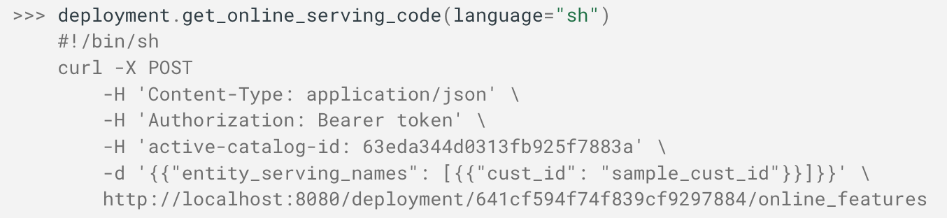
Batch serving is supported by first creating a BatchRequestTable object in the SDK that lists the entity key values for which inference is needed. The BatchRequestTable is created from either a source table in the data warehouse or a view.

Batch features values are then obtained in the SDK from the Deployment object and the BatchRequesTable. The output is a BatchFeatureTable that represents the batch features values stored in the feature store and contains metadata offering complete lineage on how the table was produced.

SDK Reference

Refer to the BatchRequestTable and BatchFeatureTable main pages or to the specific links:

get Python or shell script templates to serve a feature list online,
create an batch request table from a source table,
create an batch request table from a view,
generate batch features values,
list batch request tables and batch feature tables in a catalog,
get a batch request table or batch feature table from a catalog,
and get a batch request table or batch feature table by its Object ID from a catalog.

User Interface

Learn by example with our 'Deploy and serve a feature list' UI tutorials.

Feature List Governance¶

Feature List Version¶

The Feature List Version allows using each feature's latest version. Upon creation of a new feature list version, the latest default versions of features are employed unless particular feature versions are specified.

SDK Reference

How to:

create a new feature list version,
list versions for a feature list,
get a specific version of a feature list from a catalog,

Default Feature List Version¶

The 'Default Version of a Feature List' must comprise the default version of each feature, as indicated by its default_feature_fraction property being equal to 1. If this fraction is less than 1, a new feature list version must be created as the Default Feature List Version. Upon creation of this new list, the default_feature_fraction of the Default Feature List Version will be reset to 1.

SDK Reference

How to:

Feature List Status¶

Feature lists can be assigned one of five status levels to differentiate between experimental feature lists and those suitable for deployment or already deployed.

"DEPLOYED": Assigned to feature list with at least one deployed version.
"TEMPLATE": For feature lists as reference templates or safe starting points.
"PUBLIC_DRAFT": For feature lists shared for feedback purposes.
"DRAFT": For feature lists in the prototype stage.
"DEPRECATED": For outdated or unnecessary feature lists.

Note

The status is managed at the namespace level of a Feature List object, meaning all versions of a feature list share the same status.

For the following scenarios, some status levels are automatically assigned to feature lists:

when a new feature list is created, the "DRAFT" status is assigned to the feature list.
when at least one version of the feature list is deployed, the "DEPLOYED" status is assigned.
when deployment is disabled for all versions of the feature list, the "PUBLIC_DRAFT" status is assigned.

Additional guidelines:

Before setting a feature list status to "TEMPLATE", ensure all features in the default version are "PRODUCTION_READY".
Only "DRAFT" feature lists can be deleted.
You cannot revert a feature list status to a "DRAFT" status.
Once a feature list is in "DEPLOYED" status, you cannot update the status to other status until all the associated deployments are disabled.

SDK Reference

How to:

get the status of a feature list,
change the status of a feature list.

Feature List Readiness¶

The Feature List Readiness metric provides a statistic on the readiness of features in the feature list version. This metric represents the percentage of features that are production ready within the given feature list.

Important

Before a feature list version is deployed, all its features must be "production ready" and the metric should be 100%.

SDK Reference

How to get the readiness metric of a feature list.

Feature List Percentage of Online Enabled Features¶

The 'Feature List Percentage of Online Enabled Features' represents the proportion of features used by at least one deployed feature list. A percentage near 1 suggests a lower cost for deploying the feature list.

Feature Table¶

A Feature Table contains historical feature values from a historical feature request that are typically produced to train or test Machine Learning models. The historical feature values can also be obtained as a Pandas DataFrame, but using a Feature Table has some benefits such as handling large tables, storing the data in the feature store for reuse, and offering full lineage.

SDK Reference

Refer to the HistoricalFeatureTable object main page.

Feature Table Creation¶

In SDK, a HistoricalFeatureTable object is created by getting historical features from a feature list by using the compute_historical_feature_table() method. The method uses as input an observation table that combines historical points-in-time and key values of the feature list's primary entity or of its related serving entities.

In FeatureByte Enterprise User Interface, a Feature Table can be generated by selected a feature list and specifying an observation table compatible with the feature list.

SDK Reference

How to compute feature table.

Feature Table Lineage¶

The Feature Table contains metadata on the Feature List and Observation Table used.

SDK Reference

How to:

to access the feature_list_id
to access the observation_table_id

Feature Table Purpose¶

The purpose of a Feature Table depends on the purpose of the observation table it comes from. It can vary from being a simple preview to being used for more complex tasks like exploratory data analysis, training, or validation tests. This classification helps in easily identifying and reusing Feature Tables.

Feature Table Association with a Context or Use Case¶

The association of a Feature Table with specific Contexts or Use Cases is determined by its originating observation table. This link makes it straightforward to organize and locate Feature Tables relevant to particular use cases.

SDK Reference

How to list feature tables related to a Use Case

Deployment¶

In FeatureByte, a Deployment object manages the online and batch serving of a deployed FeatureList for specific Use Cases.

Enabling and Disabling Deployments¶

A Deployment Object is initiated when a FeatureList is deemed ready for production deployment.

Upon creation, the Deployment can be enabled for online and batch serving, triggering the orchestration of feature materialization into the online feature store.

Deployments can be disabled at any time, ceasing the online and batch serving of the feature list without impacting serving of the historical requests. This approach is distinct from the 'log and wait' method used in some other feature stores.

Note

If the feature list is associated with multiple deployments (for different use cases), disabling one deployment will not affect the serving of other deployments.

SDK Reference

Refer to the Deployment main page or to the specific links:

Deployment and Online Serving¶

For online serving, Deployment objects offer Python or shell script templates for REST API services.

SDK Reference

How to get Python or shell script templates

Deployment and Batch Serving¶

Batch serving utilizes the SDK's compute_batch_feature_table() method, returning a BatchFeatureTable object that represents a table in the feature store with batch feature values.

SDK Reference

For more details, refer to the SDK reference for BatchFeatureTable object.

Feature Job Status¶

The Deployment object provides reports on recent activities of scheduled feature jobs, including run history, success status, and durations.

In cases of failed or late jobs, it's advised to review data warehouse logs for insights, especially if the issue relates to compute capacity.

SDK Reference

How to get the feature job status for a feature list.

Deployment Catalog¶

Deployments can be associated with specific Use Cases, and all related deployments can be managed and listed from the Use Case.

SDK Reference

How to list deployments related to a Use Case

Within the catalog, deployments can be listed, retrieved by name, or by Object ID.

SDK Reference

How to:

list deployments available in a catalog,
get an a deployment from a catalog,
and get an deployment by its Object ID from a catalog.

The Deployment object class methods allow for listing and managing deployments across all catalogs.

SDK Reference

How to:

list() to list all deployments across catalogs.
get() to get an Deployment object by its name.
get_by_id() to get a Deployment object by its Object ID.

Approval Flow¶

Enabling Approval Flow¶

FeatureByte Enterprise catalogs can incorporate an Approval Flow. When active, key actions require approval such as:

Marking a feature as Production-Ready
Changing a table's Cleaning Operations,
Changing a table's Defaut Feature Job Setting.

To check if Approval Flow is active, look for a validation mark next to the Catalog name.

Name

If it's missing, click the settings icon near the Catalog name at the top of the screen to access and enable the Approval Flow option.

Name

Feature Adjustments¶

When table metadata changes occur (e.g., new cleaning operations, updating feature job settings), they trigger new feature versions. This ensures compatibility with new data. Users can modify default actions for these features and analyze the impact of both original and updated operations.

Name

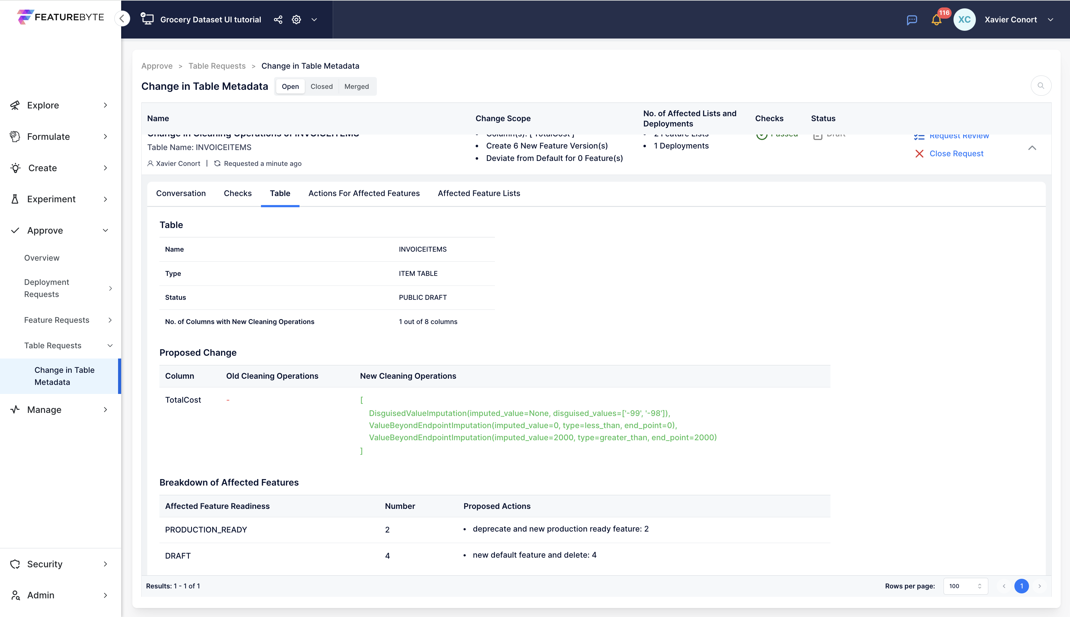
Approval Flow Checks¶

Approval Flow involves several automated checks:

For Marking a Feature as Production-Ready:

Compliance with default cleaning operations and feature job setting of its source tables.
Table status assessment
Recent analysis of data availability and freshness.
Backtesting to avoid training-serving inconsistencies.

Name

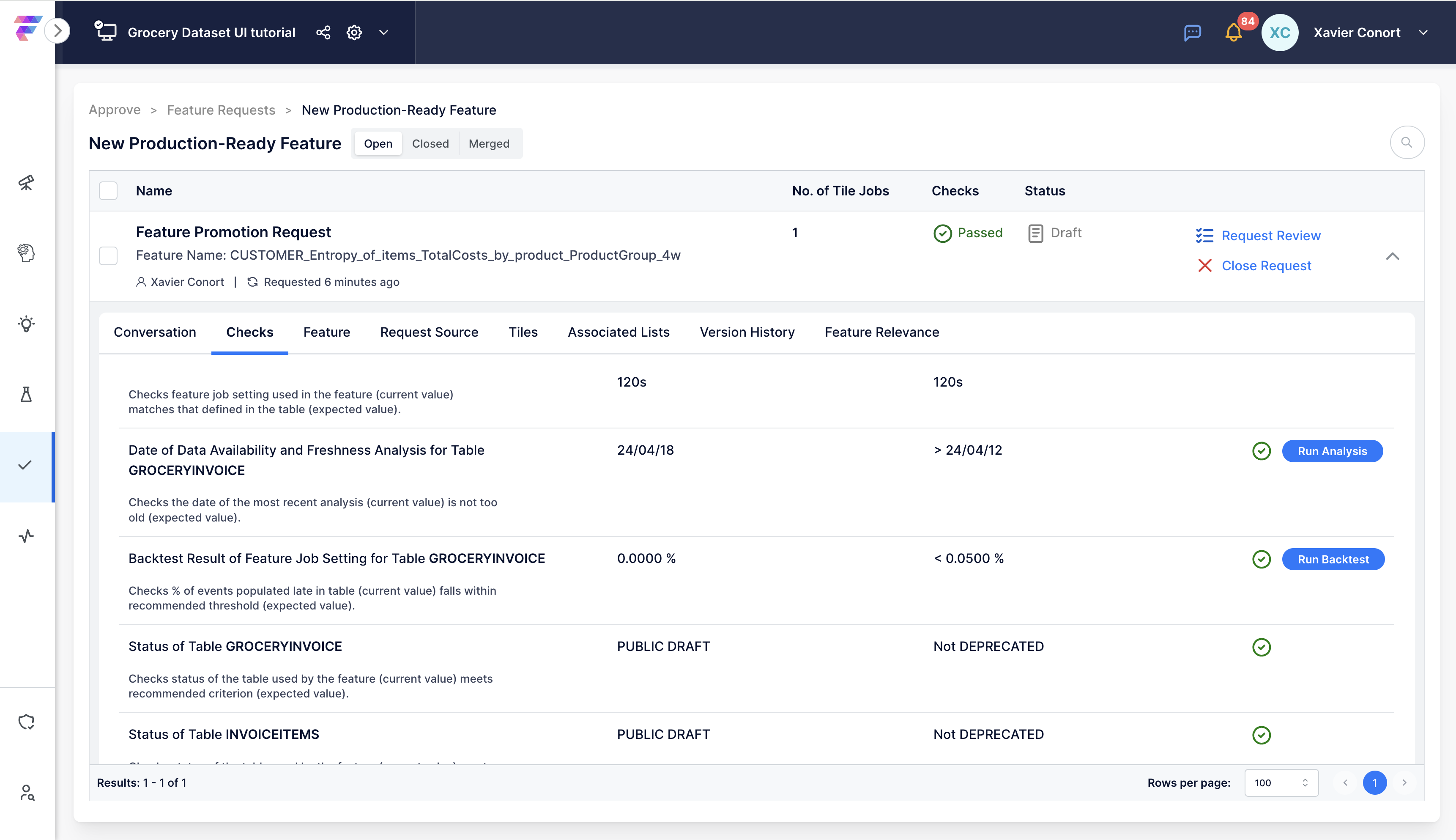
For Changes in Cleaning Operations:

Analysis of features with actions diverging from new operations.
Completion of this analysis changes request checks to green.
Emphasis on understanding impacts of both new and original operations.

Name

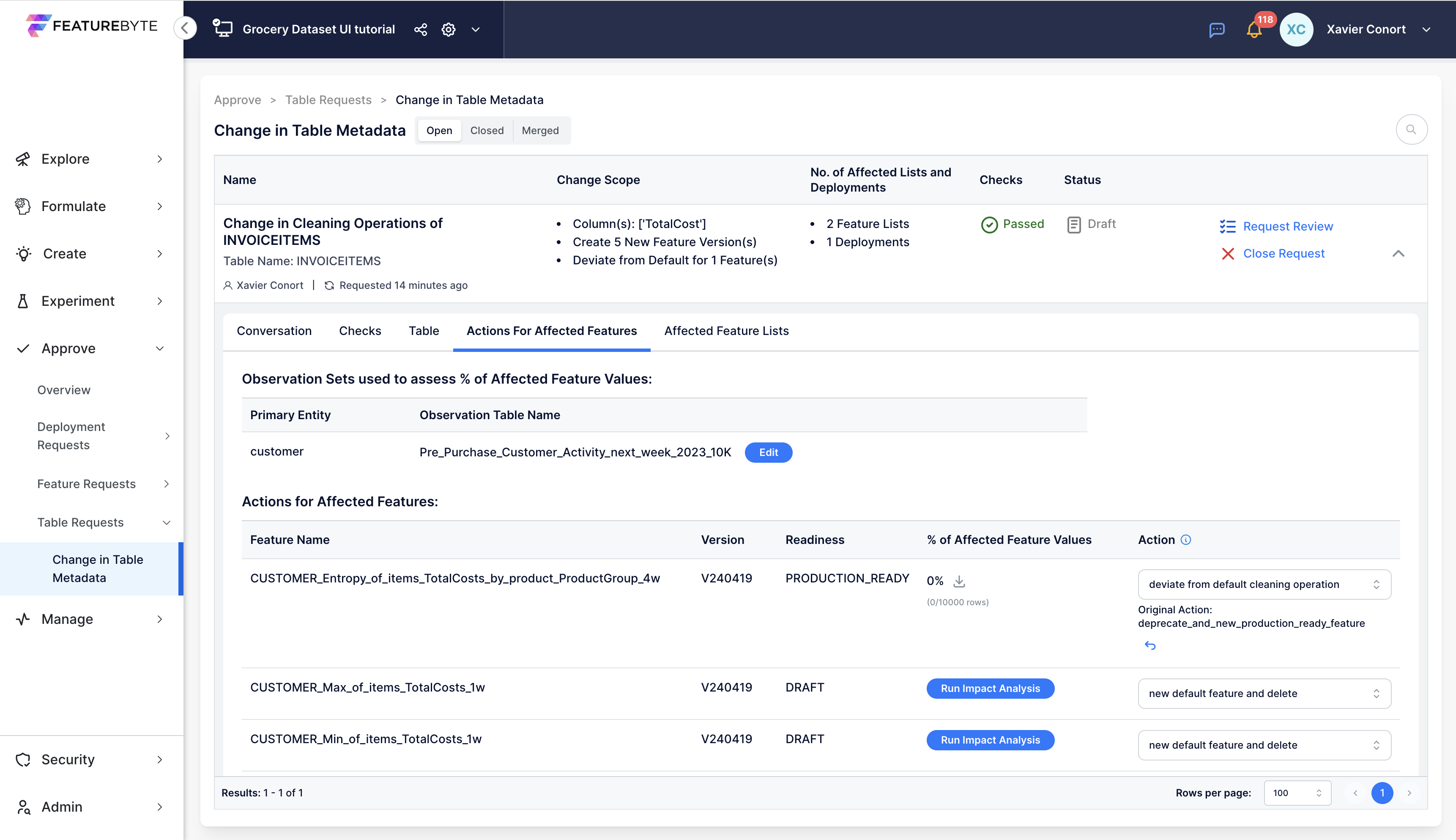
For Changes in Feature Job Setting:

Recent analysis of data availability and freshness.
Backtesting of the new setting to prevent future training-serving inconsistencies.

Name

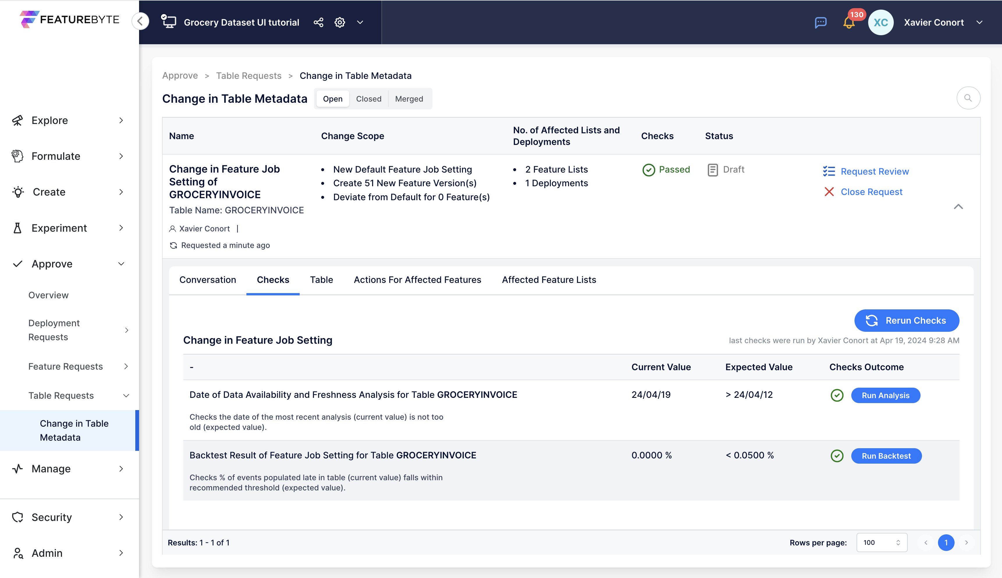
Learning Through UI Tutorials¶

For a practical understanding of the approval flow, explore our UI tutorials:

Feature Store¶

The purpose of a Feature Store is to centralize pre-calculated values, which can significantly reduce the latency of feature serving during training and inference.

FeatureByte Feature Stores are designed to integrate seamlessly with data warehouses, eliminating the need for bulk outbound data transfers that can pose security risks. Furthermore, the computation of features is performed in the data warehouse, taking advantage of its scalability, stability, and efficiency.

Pre-calculated values for online and batch serving are stored in an online feature store.

Partial aggregations in the form of online and offline tiles are also stored to streamline feature materialization for historical request and online and batch serving. This approach enables computation to be performed incrementally on tiles rather than the entire time window, leading to more efficient resource utilization.

Once a feature is deployed, the FeatureByte service automatically initiates materialization of feature and tiles, scheduled based on the feature job setting of the feature.

SDK Reference

Refer to the FeatureStore object main page or to the specific links:

Tiles¶

Tiles are a method of storing partial aggregations in the feature store, which helps to minimize the resources required to fulfill historical and online requests. There are two types of tiles managed by FeatureByte: offline tiles and online tiles.

When a feature has not yet been deployed, offline tiles are cached following a historical feature request to reduce the latency of subsequent requests. Once the feature has been deployed, offline tiles are computed and stored according to the feature job setting.

The tiling approach adopted by FeatureByte also significantly reduces storage requirements compared to storing offline features. This is because tiles are more sparse than features and can be shared by features that use the same input columns and aggregation functions.

Feature Jobs¶

Feature Job Background¶

FeatureByte is designed to work with data warehouses that receive regular data refreshes from operational sources, meaning that features may use data with various freshness and availability. If these operational limitations are not considered, inconsistencies between offline requests and online and batch feature values may occur.

To prevent such inconsistencies, it is crucial to synchronize the frequency of batch feature computations with the frequency of source table refreshes and to compute features after the source table refresh is fully completed. In addition, for historical serving to accurately replicate the production environment, it is essential to use data that would have been available at the historical points-in-time, considering the present or future data latency. Latency of data refers to the time difference between the timestamp of an event and the timestamp at which the event data is accessible for ingestion. Any period during which data may be missing is referred as a "blind spot".

To address these challenges, the feature job setting in FeatureByte captures information about the frequency of batch feature computations, the timing of the batch process, and the assumed blind spot for the data. This helps ensure consistency between offline and online feature values and accurate historical serving that reflects the conditions present in the production environment.

Feature Job¶

A Feature Job is a batch process that generates both offline and online tiles and feature values for a specific feature before storing them in the feature store. The scheduling of a Feature Job is determined by the feature job setting associated with the respective feature.

Feature job orchestration is initiated when a feature is deployed and continues until the feature deployment is disabled, ensuring the feature store consistently possesses the latest values for each feature.

Feature Job Setting¶

The Feature Job Setting in FeatureByte captures essential details about batch feature computations for the online feature store, including the frequency and timing of the batch process, as well as the assumed blind spot for the data. This helps to maintain consistency between offline and online feature values and ensures accurate historical serving that reflects the production environment.

The setting comprises of three parameters:

The frequency parameter that specifies how often the batch process should run.
The time_modulo_frequency (or offset) parameter that defines the timing from the end of the frequency time period to when the feature job commences. For example, a feature job with the following settings (frequency 60m, time_modulo_frequency: 130s) will start 2 min and 10 seconds after the beginning of each hour: 00:02:10, 01:02:10, 02:02:10, …, 15:02:10, …, 23:02:10.
The blind_spot parameter that sets the time gap between feature computation and the latest event timestamp to be processed.

Case study: A data warehouse refreshes each hour. The data refresh starts 10 seconds after the hour and is usually finished within 2 minutes. However, sometimes the data refresh misses the latest data, up to a maximum of the last 30 seconds at the end of the hour. Therefore the feature job settings will be:

frequency: 60m
time_modulo_frequency (or offset): 10s + 2m + 5s (a safety buffer) = 135s
blind_spot: 30s + 10s + 2m + 5s = 165s

In order to deal with changes in the management of the source tables where the features are sourced from, which could affect the availability or the freshness of the data, a new version of the feature can be created with updated feature job settings.

While Feature Jobs are primarily designed to support online requests, this information is also used during historical requests to minimize offline-online inconsistency.

To ensure consistency of Feature Job Setting across features created by different team members, a Default Feature Job Setting is defined at the table level. However, it is possible to override this setting during feature declaration.

SDK Reference

How to declare a feature job setting.

In feature job settings, a "blind spot" describes the time gap between the calculation of a feature and the timestamp of the most recent event included in that calculation. Ensuring that the data used in inference is complete and considering this data latency during training are key for maintaining consistency between training and serving. "Data latency" refers to the time taken from the occurrence of an event to when its data becomes usable. For data ingestion, a blind spot signifies any period where data might be missing, particularly in relation to when data ingestion is completed. Specifically, in feature computation, this blind spot extends from the end of data ingestion in the data warehouse to the beginning of the feature computation job.

The existence of this gap can affect the timeliness and relevance of data used for inference. However, maintaining a balance is important; the gap shouldn't be too brief, to preserve consistency between training and serving.

Default Feature Job Setting¶

The Default Feature Job Setting establishes the default setting used by features that aggregate data in a table, ensuring consistency of the Feature Job Setting across features created by different team members. While it is possible to override the setting during feature declaration, using the Default Feature Job Setting simplifies the process of setting up the Feature Job Setting for each feature.

To further streamline the process, FeatureByte offers automated analysis of an event table record creation and suggests appropriate setting values.

Important Note for FeatureByte Enterprise Users

In Catalogs with Approval Flow enabled, changes in table metadata initiate a review process. This process recommends new versions of features and lists linked to these tables, ensuring that new models and deployments use versions that address any data issues.

SDK Reference

How to:

User Interface

Learn by example with our 'Manage feature life cycle' UI tutorials.

Feature Job Setting Recommendations¶

FeatureByte automatically analyzes data availability and freshness of an event table to suggest an optimal setting for scheduling Feature Jobs and associated Blind Spot information.

This analysis relies on the availability of record creation timestamps in the source table, typically added when updating data in the warehouse. Additionally, the analysis focuses on a recent time window, such as the past four weeks.

FeatureByte estimates the data update frequency based on the distribution of time intervals among the sequence of record creation timestamps. It also assesses the timeliness of source table updates and identifies late jobs using an outlier detection algorithm. By default, the recommended scheduling time takes late jobs into account.

To accommodate data that may not arrive on time during warehouse updates, a blind spot is proposed for determining the cutoff for feature aggregation windows, in addition to scheduling frequency and time of the Feature Job. The suggested blind spot offers a percentage of late data closest to the user-defined tolerance, with a default of 0.005%.

To validate the Feature Job schedule and blind spot recommendations, a backtest is conducted. You can also backtest your custom settings.

SDK Reference

How to:

Feature Job Setting Backtest¶

A backtest in feature job settings evaluates the effectiveness of these settings with respect to the availability and freshness of data. This process involves calculating the proportion of new data that would have been missed in the computation of a feature if these settings had been used in previous calculations. Here, "new data" refers to data processed during the latest time frame that matches the job's frequency.

A percentage higher than 0 indicates potential future problems with training-serving consistency, as it implies that serving might utilize incomplete data.

Common reasons for backtest failures include:

Misalignment of Frequencies: The frequency at which feature jobs run should ideally be a multiple of the data warehouse's update frequency. This alignment ensures that each feature job incorporates the most recent data updates.
Premature Feature Job Start: Starting a feature job too early, before the data warehouse update is complete, can lead to incomplete data incorporation. To avoid this, set a larger offset after the completion of the data warehouse update, allowing enough time for all data to be processed.
Inadequate Data Latency Handling: Failing to account for an adequate blind spot period, the time necessary to cover data latency, can result in using incomplete data for serving. This blind spot should be long enough to ensure that all relevant data has been updated and is ready for use.
Data Warehouse Update Issues: Issues such as past failures or irregular updates in the data warehouse can also lead to backtest failures. If these issues are identified, it's important to assess whether they are likely to recur and to adjust settings or processes accordingly.

SDK Reference

How to backtest a custom feature job setting.

Training-Serving Inconsistency¶

Training-Serving Inconsistency (or Training-Serving Skew) is a difference between performance during training and performance during serving. This skew can be caused by:

A discrepancy between how you handle data in the training and serving pipelines.
A change in the data between when you train and when you serve.

This inconsistency can lead to unexpected and potentially erroneous predictions.

Data Ontology¶

FeatureByte’s Ontology is organized as a hierarchical tree, where each node represents a semantic type equipped with specific feature engineering practices. This structure facilitates understanding data characteristics and selecting appropriate processing techniques.

Data Ontology Key Concepts¶

Inheritance: Child nodes inherit feature engineering practices from their parent nodes.
Levels of Specificity: The Ontology is divided into levels, each providing a finer degree of specificity:
- Level 1: Basic generic semantic types.
- Level 2 & 3: More precise semantics for advanced feature engineering.
- Level 4: Domain-specific nodes.

Level 1 Nodes¶

unique_identifier type: Identifies each record uniquely, such as user IDs or serial numbers. Typically related to primary and foreign keys.
numeric type: Data with numerical values applicable for statistical operations like mean and standard deviation. Excludes integers used as category labels.
ambiguous_numeric type: Numeric data with uncertainties in meaning or units, requiring standardization before analysis. For instance, temperature data recorded in Fahrenheit and in Celsius require standardization to a common unit.
binary type: Data with two distinct values.
categorical type: Data with a finite set of categories, represented as integers or strings.
ambiguous_categorical type: Categorical data that might have unclear or overlapping definitions, necessitating cautious interpretation. An example is city names that are not accompanied by their state or country, leading to confusion due to the existence of multiple cities with identical names across various regions. Another example is when records are entered in various formats that may lead to ambiguity and inconsistency in how city names are recorded.
text type: Textual data, requiring complex processing such as natural language processing.
date_time type: Data representing dates and times, often requiring more precise semantic understanding for processing.
coordinates Type: Geographic data, typically latitude and longitude values.
unit type: Data indicating units of measurement.
converter type: Data used to convert or map between different units or types. For instance, conversion rates between currencies.
list type: Data presented in a list format, containing multiple items.
dictionary type: Data in a key-value pair format.
sequence type: Similar to list, but with an emphasis on the order of elements.
non_informative type: Data with minimal analytical value. Also can be used to manually indicate data which should not be used for feature engineering.

Important

Level 1 are often not precised enough to guide feature engineering. Some level 1 types such as numeric, categorical, text, date_time or coordinates can't be used to tag columns.

Nodes of the unique_identifier type¶

Most of nodes of level 2 for the unique_identifier type are identified during the table registration process. This includes event_id, item_id, dimension_id, scd_surrogate_key_id and scd_natural_key_id. The remaining type not identified during the table registration process is foreign_key_id.

Nodes of the numeric type¶

For the numeric type, the nodes of level 2 mostly determine whether:

sum can be used,
and circular statistics should be used

Its nodes of level 2 are:

non_additive_numeric type: for which mean, max, min and standard deviation are commonly used but sum is excluded. An example of non-additive numeric is customers’ ages.
semi_additive_numeric type: for which sum aggregation is recommended only at a point in time. Examples include an account balance or a product inventory
additive_numeric type: for which sum aggregation is recommended, in addition to mean, max, min and standard deviation. An example of additive numeric is customer payments for purchases.
inter_event_distance type: for which sum aggregation can be done unlike common distance which may be categorized as non_additive_numeric.
inter_event_time type: This data type is suitable for applying clumpiness metrics to measure behavior, such as binge-watching patterns. Using sum aggregation may not yield meaningful insights as it will lead to the sum of the window aggregation, unless data is filtered and the type is further categorized like inter_event_moving_time (a node of level 3). An example of when summing a column with inter_event_moving_time semantics is meaningful is when analyzing traveled time.
circular type: for which circular statistics are usually needed. Examples of data fields of a circular type include time of a day, day of a year, and direction.

Examples of Nodes of levels 3:

Examples connected to Non-Additive Numeric type include:

Measurement of Intensity (such as temperature, sound frequency, item price, …): for which change from prior value may be derived.

Examples connected to Additive Numeric type include:

non_negative_amount: for which stats grouped by categorical columns may be applied (bucketting).

Examples of nodes of level 4:

patient_temperature: for which categorization into ranges such as low, normal, fever may be derived.
patient_blood_pressure: for which categorization into ranges such as hypotension, normal, hypertension may be derived.

Nodes of the categorical type¶

The nodes of level 2 determine whether the Categorical field is an ordinal type. In this case, min, median, max mode may be applied in addition to other features commonly extracted from nominal_categorical fields.

Examples of nodes of level 3:

Important nodes of level 3 determine whether the Categorical field is an event_status or event_type.

In the presence of event_status type, subsetting data for each event_status is strongly recommended.
In the presence of event_type type, subsetting data for each event_type is also part of the best practices.

Examples of nodes of level 4:

The domain specific nodes of level 4 inform on further feature engineering that may be required:

for a ICD-10-CM: extracting the first 3 symbols may be useful

Nodes of the `text` type¶

The nodes of level 2 determine whether the text field is an special_text type, a long_text or a numeric_with_unit.

Examples of nodes of level 3:

Examples connected to Special Text include street_address, url, email, name, phone_number or software_code. Those may trigger special transformations based on their types.

The nodes of level 3 connected to long_text include review, twitter, resume or description.

Nodes of the `coordinates` type¶

Nodes of level 2 determine whether the column is a local_longitude, local_latitude, longitude or latitude. Approximation or simple operations such as mean may be possible for the local types.

Nodes of level 3 determine if the coordinates correspond to the coordinates of a moving object. This could trigger stats on speed or other movement related measures.

Nodes of the `date_time` type¶

Nodes of level 2 determine whether the column is a special column related to the table type or is associated with another field of the data.

Table-specific date_time types are:

event_timestamp
record_creation_timestamp
scd_effective_timestamp
scd_end_timestamp
iot_sensor_timestamp
time_series_date
time_series_timestamp

Other types of level 2 include timestamp_field, date_field and year.

Examples of nodes of level 3:

date_of_birth: Important to derive age and further age related features.
start_date: When this semantic is detected in a SCD table, it can be used to create recency features.
termination_date: When this semantic is detected in a SCD table, it can be used to subset data to create count features as a point in time.

Nodes of the `ambiguous_numeric` type¶

The nodes of level 2 determine whether the ambiguous_numeric field is of mixed_unit_numeric type.

Examples of nodes of level 3:

mixed_unit_numeric, mixed_currency_amount, mixed_unit_length, mixed_unit_time, mixed_unit_weight, mixed_unit_volume, mixed_unit_area, mixed_unit_speed, or mixed_unit_temperature.

Nodes of the `unit` type¶

The nodes of level 2 determine whether the unit field is a currency, length_unit, time_unit, weight_unit, volume_unit, area_unit, speed_unit or temperature_unit.

Nodes of the `converter` type¶

The nodes of level 2 determine whether the converter field is a fx_rate.

Nodes of the `list` type¶

The nodes of level 2 determine whether the list field is a categorical_list, text_list or numeric_list.

Nodes of the `dictionary` type¶

The nodes of level 2 determine whether the dictionary field is a dictionary_of_non_positive_calues, dictionary_of_non_negative_values or dictionary_of_unbounded_values.

Nodes of the `sequence` type¶

The nodes of level 2 determine whether the list field is a categorical_sequence, text_sequence or numeric_sequence.